[ Printable poster (pdf, 5.3M) ]
For abstract, location(s) and registration see
https://agenda.infn.it/event/20980/
- Lecture 1 (8 January)
- Slides:
References, links, etc.
- Lecture 2 (15 January)
- Slides:
-
wls_02.pdf
(with recommended homework(*))
[(*) Suggested addendum on the AIDS problem:
make a sensitivity study changing the
prior probability of infected by
±10%, ±20% and ±50%.
]
References, links, etc.
- C'è statistica e statistica, Scaffali di SxT, 30 marzo 2005 (pdf;
copia locale).
- When ISTAT tries to explain Bayesian reasoning:
- Teaching statistics in the physics curriculum.
Unifying and clarifying role of subjective probability,
AJP 67, issue 12 (1999) 1260-1268;
arXiv:physics/9908014
[Limited
to Sections I-IV, for the moment]
- More lessons from the six box toy experiment,
arXiv:1701.01143.
- Constraints on the Higgs Boson Mass from Direct Searches and Precision Measurements, by GdA and G. Degrassi,
arXiv:hep-ph/9902226
updated: Constraining the Higgs boson mass through the combination of direct search and precision measurement results,
arXiv:hep-ph/0001269.
- Bayesian reasoning versus conventional statistics in High Energy Physics,
arXiv:physics/9811046
- Hugin
(Graphical User Interface; Samples)
- Ready-to-use models based on the six-boxes toy experiment:
- Try to edit the models
(within HUGIN), changing the probability
tables, adding nodes, etc..
- Try to write from scratch the (minimalist) model to solve
the AIDS problem, using the number suggested in the slides
for easy comparisons.
just two nodes
- Infected, with two possible states,
Yes and No;
- Analysis result, with two possible states,
Positive/ and Negative.
- Modify the previous model, using equiprobable
priors for Infected/Non-Infected:
- compare the result with the those obtained
with (roughly) realistic priors;
- compare the result with the wrong one suggested
in the first lecture.
- Think then to the possible practical utility of
using equiprobable priors.
- An interesting classical example
is the so called `Asia':
(Indeed, a valid, for some aspects even better, alternative to Hugin is provided
by Netica, also
thank to the many available
tutorials
examples
whose interest goes beyond the specific package.)
- Lecture 3 (22 January)
- Slides:
- wls_03.pdf
(with recommended homework)
- Extra (very important!) problems in order
to understand meaning and role of probabilistic dependence/independence.
(We shall return on the topic in the context
of correlation coefficients)
- More on the distribution of the
product of the outcomes of two dice:
Alternative way to produce the histogram:
outcomes = as.vector(outer(1:6,1:6))
hist(outcomes, nc=40, freq=FALSE, col='cyan', xlab='x', ylab='f(x)')
- Then, here is out to make a random generator following the distribution:
sample(outcomes, 100, rep=TRUE)
(For help on the R functions you che use, e.g., ?sample, or search on the web.)
References, links, etc.
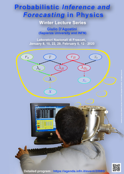
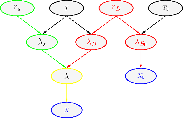
Now we are finally ready to analyze the
graphical model of the lectures poster.
Additional homework based on
the diagram:
- prove, just using physics arguments, that
λ = λS + λB;
- then, using the reasoning used in the previous item,
draw the diagram in a different, more physical, way.
- Lecture 4 (29 January)
-
Slides:
- wls_04.pdf
(with recommended homework)
“Probability
is the very guide of life”
Remarks: as announced in advance by mail, this lecture contained
also several technical aspects `just mentioned'. In particular
- slides 85-89 were meant as a kind of euristic way
to arrive to the general expression of the
multivariate normal distribution;
- slide 90 is a summary concerning covariance matrix
and correlation matrix;
- slide 91 contains a warning analogue to that of slide
19;
- slides 92-100 is a reminder concerning propagation
of uncertainties in linear combination also taking into account
covariances, leading to the (should be) well known
'transformations of covariance matrix'
VY = C VX CT;
Note: when the transformation is not linear, although
linearized (pay attention!) the matrix C
contains derivatives, as quite well known
(subject not covered in the lectures);
- finally, pp. 102-104 are (for the moment) suggestions
for self study
to those interested in the subject,
discussed at length in arxiv:1504.02065.
References, links, etc.
- Gauss, Theoria Motus Corporum Coelestium in Sectionibus Conicis Solem Ambientium,
SECTIO TERTIA,
pp. 205-224 (expecially p. 212).
- Gauss, Theory of the motion of the heavenly bodies moving about the sun in conic sections,
Third Section, pp. 249-273 (expecially pp. 258-259).
- Dispense "Probabilità e incertezze di misura"
(in Italian, but you might recognize the formulae of the slides)
- Parte 2:
8.1-8.8, 8.11, 8.14.3.
- Parte 3:
9.1-9.7, 9.10-9.11; 10.5, 10.7-10.14.
- Asymmetric Uncertainties: Sources, Treatment and Potential Dangers,
arXiv:physics/0403086.
- Learning about probabilistic inference and forecasting by playing with multivariate normal distributions, arxiv:1504.02065, limited to Section 2..
- Central Limit Theorem at work
Once R is installed (there are plenty of tutorials on the web),
a script can be executed by the command 'source()',
e.g. source("sum_Z2.R")
Extra work suggested in view of the following lectures
(we have something Laplace and Gauss did not have...)
- Install JAGS
and rjags (free and multiplatform).
(Those who use Python might want to use pyjags)
- Some simple examples
- simple_simulations.R
JAGS is `improperly' used as random generator,
to generate quantities following normal, binomial, Poisson and
exponential distributions.
- simple_network.R
More interesting case (but without realistic physical meaning) in which a variable can be a parameter
of the distribution of another variables.
Exercise: write the diagram connecting the four variable.
- first_inference.R
We have observed x successes in n trials: what is the Bernoulli
parameter p? (Try to change the values, including x=0 and x=n)
(For the moment it looks magics...)
- Make a variation of the previous model adding to the
inference of p also the
prediction of the number of successes in future trials, assuming
that the Bernoulli parameter p remains constant (although uncertain in value):
- add the variable xf ('f' for future)
following a binomial distribution with p and
nf;
- draw the diagram of the model;
- run the modified script, varying n, x and nf and observing the results about
p and xf, in order to get an intuition of what is going on;
- in order to get an idea of what JAGS is doing,
write (on paper) the joint distribution
f(x,n,p,xf,nx) using the chain rule, choosing the most
useful chain.
(Pag. 65 of today's slides can help.)
- Lecture 5 (5 Febuary)
- Slides:
- wls_05.pdf
(with recommended homework)
- Extended graphical model,
also including the time distribution
between two consecutive events
due to either signal or background.
- Scripts shown in the slides:
References, links, etc.
Homework
- Write the JAGS model of
graphical model of the poster.
(Use uniform priors for rS vs rB via suitable gamma distributions)
- Run it with following data:
data = list(X=100, T=10, TB=4, XB=20)
(Note: T and TB are given in unit of time, which
might be arbitrary but the same for both variables
and it will be reflected into the units
of rS vs rB.)
- At the end of the sampling
- make the summary and the summary plots as shown in the example
scripts;
- convert the histories of rS and of rB
into 'vectors';
- draw the histograms of the two variables;
- calculate averages, standard deviations and correlation
coefficient.
- draw the scatter plot of rS vs rB.
- Then, finally:
- assuming that 'we know' that the rate of background
is exactly rB=7 u (with 'u' a suitable unit),
how will this information change the value
(and the standard uncertainty) of rS?
This can be done in two ways (and it is interesting
to compare the results):
- modify the R script that calls JAGS;
- do it by a simple calculation, assuming that
f(rS,rB) is a bivariate Gaussian distribution.
- Lecture 6 (12 February)
- Slides:
- wls_06.pdf
(with recommended homework)
- JAGS/rjags script:
References, links, etc.
- About the proof of the so called exact classical confidence intervals. Where is the trick?,
arXiv:physics/0605140
- Bayesian Reasoning versus Conventional Statistics in High Energy Physics,
arXiv:physics/9811046
- Dispense "Probabilità e incertezze di misura"
(in Italian, but you might recognize the formulae of the slides)
- Parte 4: Sections
11.5, 11.6, 11.7.
- Bayesian reasoning in high-energy physics: principles and applications, Sections 5.6 (plus 6.1.1,
just mentioned during the lecture):
- Fits, and especially linear fits, with errors on both axes, extra variance of the data points and other complications,
arXiv:physics/0511182
- Laplace’s approximation for Bayesian posterior distribution
- Spurious correlations
And, obviously, much more here
Recommended exercise with JAGS:
(simulated) data samples affected by systematics of two kinds
- Code:
- Suggested work:
- write down the graphical model;
- run the script as is;
- play with the values of sigma.z and sigma.f
(if they a both zero there are no systematics);
- play with the various model parameters;
- make scatter plots among some variables that might be interesting
and calculate the correlation coefficients
(before you do it:
which quantities do you expect to be correlated and which sign of
ρ do you expect?);
- introduce in the model other derived quantities, like
products and ratios of mu1, mu2 and mu3;(*)
- write the code in order to calculate in closed formulae
(although with reasonable approximations)
the results obtained by sampling
(you can do in your preferred programming language,
using averages and standard deviations provided by the R script)
(*) Note: in reality there is no need to evaluate the 'derived
quantities', including Delta.mu.21 and Delta.mu.32, in JAGS
and they can be more conveniently calculated in the steering script
from the histories of mu1, mu2 and mu3.
Root users might want to implement the JAGS model in
BAT