Combining uncertain priors and uncertain weights of evidence
When we have set up our problem, listed the
pieces of evidence pro and con, including the 0-th one
(the prior), and attributed to each of them a weight of
evidence, quantified by the corresponding  JL's,
we can finally sum up all contributions.
JL's,
we can finally sum up all contributions.
As it is easy to understand, if the number of pieces of evidence
becomes large, the final judgment can be rather precise
and far from being perfectly balanced,
even if each contribution is weak and even uncertain.
This is an effect of the famous
`central limit theorem' that dumps
the weight of the values far from the
average.22
Take
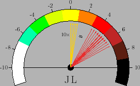
Figure:
Combined effect of
10 weak and `vague' pieces of evidence,
each yielding a JL of
 (see text).
 |
for example the case of 10 JL's each
uniformly23ranging between 0 and 1, i.e.
JL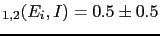 .
Each piece of evidence is marginal, but the sum leads to
a combined
JL
.
Each piece of evidence is marginal, but the sum leads to
a combined
JL of
of
 ,
where ``
,
where ``![$ [3.2,6.8]$](img227.png) '' defines now an effective range
of leanings24,
as depicted in figure 4.
Note that in this graphical representation
the 5 yellow arrows (the lighter ones if you are reading
the text in black/white)
do not represent individual values of JL,
but its interval. These arrows have all the same width
to indicate that the exact value is indifferent to us.
The red arrow have instead different widths to indicate that
we prefer the values around 5 and the preference goes down as we
move far form it. The 12 arrows only indicate an effective range,
because the full range goes from 0 to 10, although JL values
very far from 5 must have negligible weight in our reasoning.
'' defines now an effective range
of leanings24,
as depicted in figure 4.
Note that in this graphical representation
the 5 yellow arrows (the lighter ones if you are reading
the text in black/white)
do not represent individual values of JL,
but its interval. These arrows have all the same width
to indicate that the exact value is indifferent to us.
The red arrow have instead different widths to indicate that
we prefer the values around 5 and the preference goes down as we
move far form it. The 12 arrows only indicate an effective range,
because the full range goes from 0 to 10, although JL values
very far from 5 must have negligible weight in our reasoning.
Giulio D'Agostini
2010-09-30