Foreword
We have seen the use of jupyter notebooks.
As a matter of fact these slides are a notebook converted to (HTML) slides via the jupyter-nbconvert utility.
Get the code from gitlab here: https://gitlab.com/carlomt/pycourse with, in an new terminal:
git clone https://gitlab.com/carlomt/pycourse
cd pycourse
conda env create -f environment.yml
conda activate pycourse
. post-install.sh #Configure some extra stuff
The pre-installed environment course is enough to read/edit these slides.
Read the README.md file for additional instructions.
Python Introduction Course: Data Science tools
With emphasis on data-science problems
This course is available on gitlab
Contact us: andrea.dotti@gmail.com, mancinit@infn.it
The SciPy library contains several packages to perform specialized scientific calculations:
- Special functions (
scipy.special) - Integration (
scipy.integrate) - Optimization (
scipy.optimize) - Interpolation (
scipy.interpolate) - Fourier Transforms (
scipy.fftpack) - Signal Processing (
scipy.signal) - Linear Algebra (
scipy.linalg) - Sparse Eigenvalue Problems with ARPACK
- Compressed Sparse Graph Routines (
scipy.sparse.csgraph) - Spatial data structures and algorithms (
scipy.spatial) - Statistics (
scipy.stats) - Multidimensional image processing (
scipy.ndimage) - File IO (
scipy.io)
![]()
Numpy
It is the foundation of python scientific stack.
The basic building block is the numpy.array data structure. It can be used as a python list of numbers, but it is a specialized efficient way of manipulating numbers in python.
import numpy as np
a = np.array([1, 2, 3, 4], dtype=float)
a
a = range(1000)
%timeit [ i**2 for i in a]
b = np.arange(1000)
%timeit b**2
c = np.array([[1,2],[3,4]])
c
c.ndim
c.shape
c = np.arange(27)
c.reshape((3,3,3))
np.zeros((2,2))
np.ones((2,1))
a = np.arange(27).reshape((3,3,3))
np.ones_like(a)
np.eye(3)
a = np.arange(10)
a
a[0]
a[-1]
a[0:3]
a[::2]
a = a.reshape(5,2)
a
a[3,1]
a[2,:]
Important: Views or copy
A slice or reshape is a view, simply a re-organization of the same data in memory, thus changing one element changes the same element in all views
a = np.arange(9)
b = a.reshape((3,3))
np.may_share_memory(a,b)
a[3] = -1
b
b = a.copy()
np.may_share_memory(a,b)
Boolean masks for extracting values
A typical operation done in your daily physics data analysis is to extract from an array the values that match a condition. Consider an array of the energies of particles, and assume you want to use only the energies above a given threshold. Boolean masking comes at a rescue
ene = np.random.exponential(size=10, scale=10.) # 1/scale e^(-ene/scale)
ene
mask = ene > 2
mask
ene[mask]
ene[ene<2]
ene[ene<2] = 0
ene
Values with list of indexes
Similarly to boolean masks it is possible to access and modify values directly to an array using a list of indexes
status = np.random.randint(low=0,high=10,size=10)
status
status[[0, 3, 5]]
status[[0, 3, 5]] = -1
status
Simple Operations
a = np.arange(4)
a
a+1
10**a
np.sin(a)
Reductions
a = np.random.randint(low=0,high=10,size=4)
a
np.sum(a)
np.max(a), np.min(a)
np.argmax(a), np.argmin(a)
np.mean(a), np.median(a), np.std(a)
a = a.reshape(2,2)
a
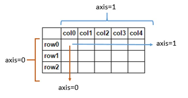
np.sum(a,axis=0)
m1 = a>0
m1
np.all(m1)
np.any(m1)
Matplotlib
Matplotlib is probably the most used Python package for 2D-graphics. It provides both a quick way to visualize data from Python and publication-quality figures in many formats.
Other visualization packages exists, often these are built on top of matplotlib.
The package is well integrated into IPython and Jupyter.
%matplotlib inline
from matplotlib import pyplot as plt
import numpy as np
X = np.linspace(-np.pi, np.pi, 256, endpoint=True)
C, S = np.cos(X), np.sin(X)
plt.plot(X,C)
plt.plot(X,S)

Customization
plt.figure(figsize=(4, 3), dpi=80)
plt.plot(X, C, color="blue", linewidth=1.0, linestyle="-", label="cos")
plt.plot(X, S, color="green", linewidth=1.0, linestyle="-", label="sin")
plt.xlim(-4.0, 4.0)
plt.xticks(np.linspace(-4, 4, 9, endpoint=True))
plt.savefig("example.png", dpi=72)
plt.grid()
plt.xlabel("x")
plt.ylabel("y")
plt.title("Example")
plt.legend(loc="best")

Multiple plots
plt.figure(figsize=(6, 4))
plt.subplot(2, 2, 1)
plt.plot(X, C, color="blue", linewidth=1.0, linestyle="-", label="cos")
plt.subplot(2, 2, 2)
plt.plot(X, S, color="green", linewidth=1.0, linestyle="-", label="sin")
plt.subplot(2, 2, 3)
plt.plot(X, C, color="red", linewidth=1.0, linestyle="-", label="cos")
plt.subplot(2, 2, 4)
plt.plot(X, S, color="black", linewidth=1.0, linestyle="-", label="sin")
plt.show()

Examples
plt.rcdefaults()
fig, ax = plt.subplots(figsize=(4,3))
# Example data
people = ('Tom', 'Dick', 'Harry', 'Slim', 'Jim')
y_pos = np.arange(len(people))
performance = 3 + 10 * np.random.rand(len(people))
error = np.random.rand(len(people))
ax.barh(y_pos, performance, xerr=error, align='center',
        color='green', ecolor='black')
ax.set_yticks(y_pos)
ax.set_yticklabels(people)
ax.invert_yaxis()  # labels read top-to-bottom
ax.set_xlabel('Performance')
ax.set_title('How fast do you want to go today?')

plt.show()

x = np.linspace(0, 1, 500)
y = np.sin(4 * np.pi * x) * np.exp(-5 * x)
fig, ax = plt.subplots()
ax.fill(x, y, zorder=10)
ax.grid(True, zorder=5)
plt.show()

fig, ax = plt.subplots()
for color in ['red', 'green', 'blue']:
    n = 750
    x, y = np.random.rand(2, n)
    scale = 200.0 * np.random.rand(n)
    ax.scatter(x, y, c=color, s=scale, label=color,
               alpha=0.3, edgecolors='none')

ax.legend()
ax.grid(True)

plt.show()

mu = 200
sigma = 25
x = np.random.normal(mu, sigma, size=100)
fig, (ax0, ax1) = plt.subplots(ncols=2, figsize=(6, 3))
ax0.hist(x, 20, density=1, histtype='stepfilled', facecolor='g', alpha=0.75)
ax0.set_title('stepfilled')
# Create a histogram by providing the bin edges (unequally spaced).
bins = [100, 150, 180, 195, 205, 220, 250, 300]
ax1.hist(x, bins, density=1, histtype='bar', rwidth=0.8)
ax1.set_title('unequal bins')
plt.title(r'Histogram of IQ: $\mu=100$, $\sigma=15$');

from matplotlib import colors, ticker, cm
from scipy.stats import multivariate_normal

N = 100
x = np.linspace(-3.0, 3.0, N)
y = np.linspace(-2.0, 2.0, N)

X, Y = np.meshgrid(x, y)
pos = np.empty(X.shape+(2,))
pos[:,:,0] = X; pos[:,:,1] = Y
# A low hump with a spike coming out of the top right.
# Needs to have z/colour axis on a log scale so we see both hump and spike.
# linear scale only shows the spike.
z = (multivariate_normal([0.1, 0.2], [[1.0, 0.],[0, 1.0]]).pdf(pos)
     + 0.1 * (multivariate_normal([1.0, 1.0],[[0.01, 0.],[0., 0.01]])).pdf(pos))
# Automatic selection of levels works; setting the
# log locator tells contourf to use a log scale:
fig, ax = plt.subplots(figsize=(4,3))
cs = ax.contourf(X, Y, z, locator=ticker.LogLocator(), cmap=cm.PuBu_r)
cbar = fig.colorbar(cs)


![]()
Pandas
Pandas is a high-performance, high-level library that provides tools for data analysis.
It relies on the concept of DataFrame: a structured collection of data organized in records. This is the same concept of ROOT's NTuple that you are familiar with.
I think the name comes from R.
import numpy as np
import pandas as pd

s = pd.Series( [1., 2., 3., np.nan, 5. ], index=["a","b","c","d","e"])
s
df = pd.DataFrame(
    {
        'Col1': [1.,2.,3.,4.],
        'Col2': ["a","b","c","d"],
        'Col3': [True, False, True, True]
    }
)
df
Reading/Saving dataframes
Pandas support reading writing to several data formats, via specialized routines, many other formats, because dataframe (with other names) are a common concept:
| Format Type | Data Description | Reader | Writer |
|---|---|---|---|
| text | CSV | read_csv |
to_csv |
| text | JSON | read_json |
to_json |
| text | HTML | read_html |
to_html |
| text | Local clipboard | read_clipboard |
to_clipboard |
| binary | MS Excel | read_excel |
to_excel |
| binary | HDF5 Format | read_hdf |
to_hdf |
| binary | Feather Format | read_feather |
to_feather |
| binary | Parquet Format | read_parquet |
to_parquet |
| binary | Msgpack | read_msgpack |
to_msgpack |
| binary | Stata | read_stata |
to_stata |
| binary | SAS | read_sas |
|
| binary | Pickle Format | read_pickle |
to_pickle |
| SQL | SQL | read_sql |
to_sql |
| SQL | Google Big Query | read_gbq |
to_gbq |
As you can see the physicists ROOT format is not natively supported. However some external software to read TTrees are available. For example root_numpy, root_pandas, or uproot. ROOT usually comes with pre-installed pyROOT library (the one on the provided VM works only for python2), that offers basic functionalities.
df.dtypes
df.columns
df.index
View data
df = pd.DataFrame( {'A':np.random.randint(0,10,100), 'B': [2**x for x in np.arange(100)], 'C':"a"})
df.head()
df.tail(2)
df.describe()
Select data
dates = pd.date_range('20190527',periods=7)
df = pd.DataFrame( np.random.rand(7,4), index=dates, columns=['A','B','C','D'])
df
df['A'] # or df.A
df[0:2]
df['20190529':'20190531']
dates
df.loc[dates[2]]
df.loc[dates[2],['B','C']]
df.iloc[2,2:4]
df[ df>0.5 ]
Setting values
s = pd.Series( np.random.rand(7), index=dates )
s
df['E'] = s
df
df.loc[:,['C']] = 0
df
Operations
df.mean()
df.mean(axis=1)
Merging dataframes
df1 = pd.DataFrame( np.random.rand(7,2), index=dates, columns=['A','B'])
df2 = pd.DataFrame( np.random.rand(7,3), index=dates, columns=['C','D','E'])
pd.concat([df1,df2],sort=False)
pd.concat([df1,df2],axis=1,join='inner')
Grouping
s = pd.Series( ["a","b","a","c","a","c","b"], index=dates)
df['E']=s
df
df.groupby('E').sum()
Pivot table
dates = pd.date_range('20190527',periods=6, name='date')
df = pd.DataFrame( np.random.rand(6,3), index=dates, columns=['A','B','C'])
df['D'] = pd.Series(["a","a","b","b","c","c"],index=dates)
df['E'] = pd.Series(["one","two","one","two","one","two"],index=dates)
df
pd.pivot_table(df, values=['A','B','C'], index=['D','E'])
Plotting data
%matplotlib inline
df.plot()
