TensorFlow

Introduction
- a free and open-source software library for dataflow and differentiable programming across a range of tasks
- symbolic math library, and is also used for machine learning applications such as neural networks
- used for both research and production at Google
- developed by the Google Brain team for internal Google use
- It was released under the Apache License 2.0 on November 9, 2015.
Disclaimer
This is not to be intended as a TensorFlow or Deep Learning class
It's just an introduction to it, to show the Python potentialities
Installing
You can install TensorFlow via pip
https://www.tensorflow.org/install/pip?lang=python3
(remember to install tensorflow-gpu instead of tensorflow if you have an NVIDIA GPU with CUDA and cuDNN installed)
or compiling it
For this course
We added tensorflow in the environment.yml file
So you already installed it with Anaconda
Keras

- Keras is an open-source neural-network library
- Written in Python
- Can run on top of TensorFlow, Microsoft Cognitive Toolkit, R, Theano, or PlaidML
- Designed to enable fast experimentation with deep neural networks
Keras and TensorFlow
In 2017, Google's TensorFlow team decided to support Keras in TensorFlow's core library
Keras is included in TensorFlow 2.0
Let's play with Keras and TensorFlow
We will start from a TensoFlow basic example
It build a fully connected Neural Network
With one hidden layer
To classify clothes from MNIST fashion!
import numpy as np
import matplotlib.pyplot as plt
import tensorflow as tf
from tensorflow import keras
Building a model
model = keras.Sequential([
    keras.layers.Flatten(input_shape=(28, 28)),
    keras.layers.Dense(units=128, activation='relu'),
    keras.layers.Dense(units=10, activation='softmax')
])
- Firstly we flatten the input
- Then a fully connected hidden layer
- with 128 neurons
- an a Rectified Linear Unit (ReLU) as activation function
- Finally another fully connected with 10 outputs (the number of classes we want to identify)
z = np.arange(-2, 2, .1)
zero = np.zeros(len(z))
y = np.max([zero, z], axis=0)

fig = plt.figure()
ax = fig.add_subplot(111)
ax.plot(z, y)
ax.set_ylim([-2.0, 2.0])
ax.set_xlim([-2.0, 2.0])
ax.grid(True)
ax.set_xlabel('z')
ax.set_title('Rectified linear unit')
Text(0.5, 1.0, 'Rectified linear unit')
Softmax takes as input a vector of n real numbers, and normalizes it into a probability distribution consisting of n probabilities proportional to the exponentials of the input numbers
prior to applying softmax:
- some vector components could be negative, or greater than 1
- might not sum to 1
after softmax:
- each component will be in the interval ( 0 , 1 ) {\displaystyle (0,1)} (0,1),
- the components will add up to 1
- the larger input components will correspond to larger probabilities
Softmax is often used in neural networks, to map the non-normalized output of a network to a probability distribution over predicted output classes.
Then we compile the model
Before the model is ready for training, it needs a few more settings. These are added during the model's compile step:
- Loss function —This measures how accurate the model is during training. You want to minimize this function to "steer" the model in the right direction.
- Optimizer —This is how the model is updated based on the data it sees and its loss function.
- Metrics —Used to monitor the training and testing steps. The following example uses accuracy, the fraction of the images that are correctly classified.
model.compile(optimizer='adam',
              loss='sparse_categorical_crossentropy',
              metrics=['accuracy'])
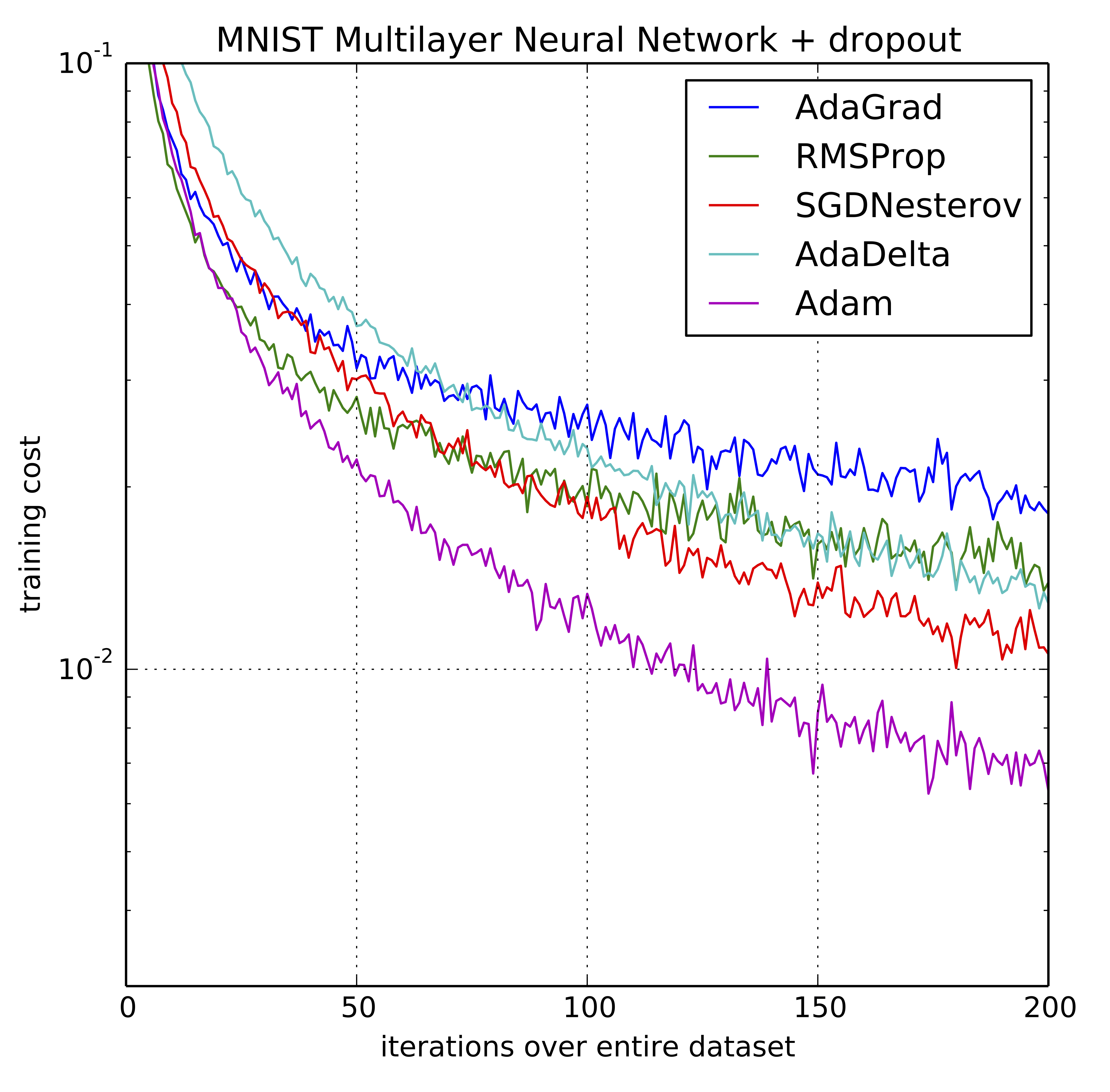
The Adam optimization algorithm is an extension to stochastic gradient descent that has recently seen broader adoption for deep learning applications in computer vision and natural language processing.
The method computes individual adaptive learning rates for different parameters from estimates of first and second moments of the gradients.
Adam adapts the learning rates using the averages of the first and second moment of the gradients
Using large models and datasets, we demonstrate Adam can efficiently solve practical deep learning problems.

And finally fit it!
Training the neural network model requires the following steps:
- Feed the training data to the model. In this example, the training data is in the
train_imagesandtrain_labelsarrays. - The model learns to associate images and labels.
- You ask the model to make predictions about a test set—in this example, the
test_imagesarray. Verify that the predictions match the labels from thetest_labelsarray.
To start training, call the model.fit method—so called because it "fits" the model to the training data:
epochs=10
history = model.fit(train_images,
                    train_labels,
                    epochs=epochs,
                    validation_data=(validation_images,validation_labels))