Next: Bibliography Up: An update of the Previous: Conclusions

Acknowledgements

Due to my service on army I could write this note only in this period even if the results shown here have been developed during the collaboration with Ludger Lindemann, and all Fsigma group, to study the

structure function with '95 SVX data. For this reason I can say, only now, thank you to all Fsigma group and to the ``young dad''.

$\begin{sidewaystable} % latex2html id marker 241 [h] {\tiny \centering \be... ...\ref{fig:bin}. The values are given in percentage. } } \end{sidewaystable}$

**Figure:** *Comparison between data (dots) and MonteCarlo( hatched histogram)*
$\begin{figure} \centerline{ \epsfig{figure=figure/show1.eps,clip=}} \end{figure}$

**Figure:** *Comparison between data (dots) and MonteCarlo( hatched histogram)*
$\begin{figure} \centerline{ \epsfig{figure=figure/show2.eps,clip=}} \end{figure}$

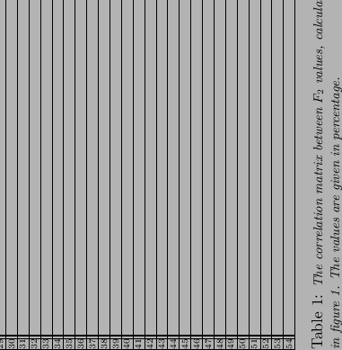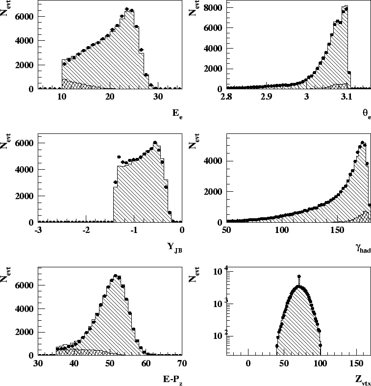**Figure:** *Results (open circle) on vs compare with the published ZEUS '95 SVX data (open diamond)*
$\begin{figure} \centerline{ \epsfig{figure=figure/f2_cfr.eps,height=20cm,clip=}} \end{figure}$

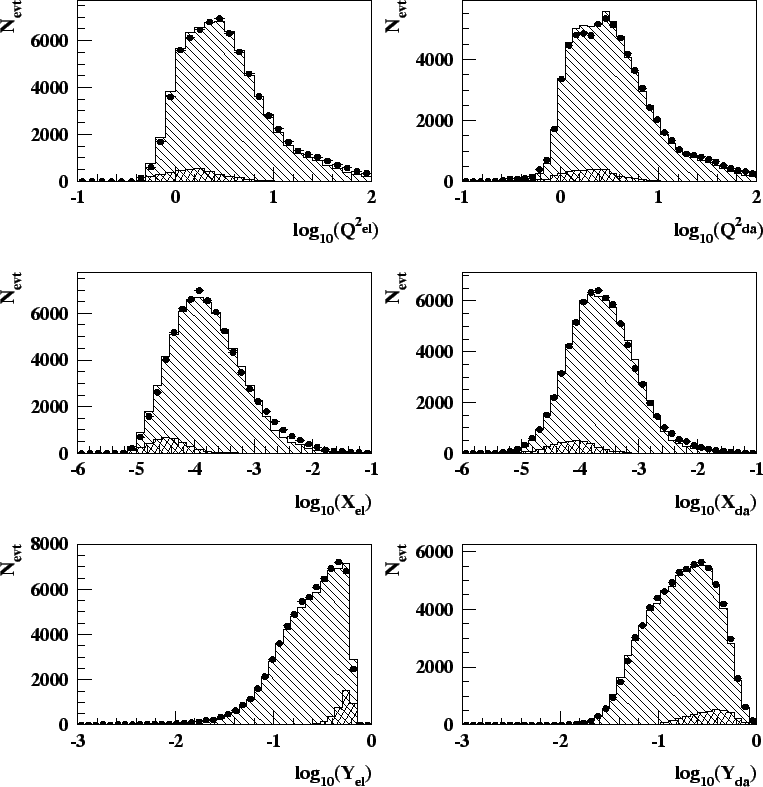**Figure:** Results (open circle) on vs compare with H1 95 (open square), ZEUS 94 (open diamond), BPC (cross) and E665,SLAC,NMC (solid circle). The solid line is the ZEUS NLO fit [3]. For the first 2 bins the uncertainties on the fit (shadow area) is shown, too.
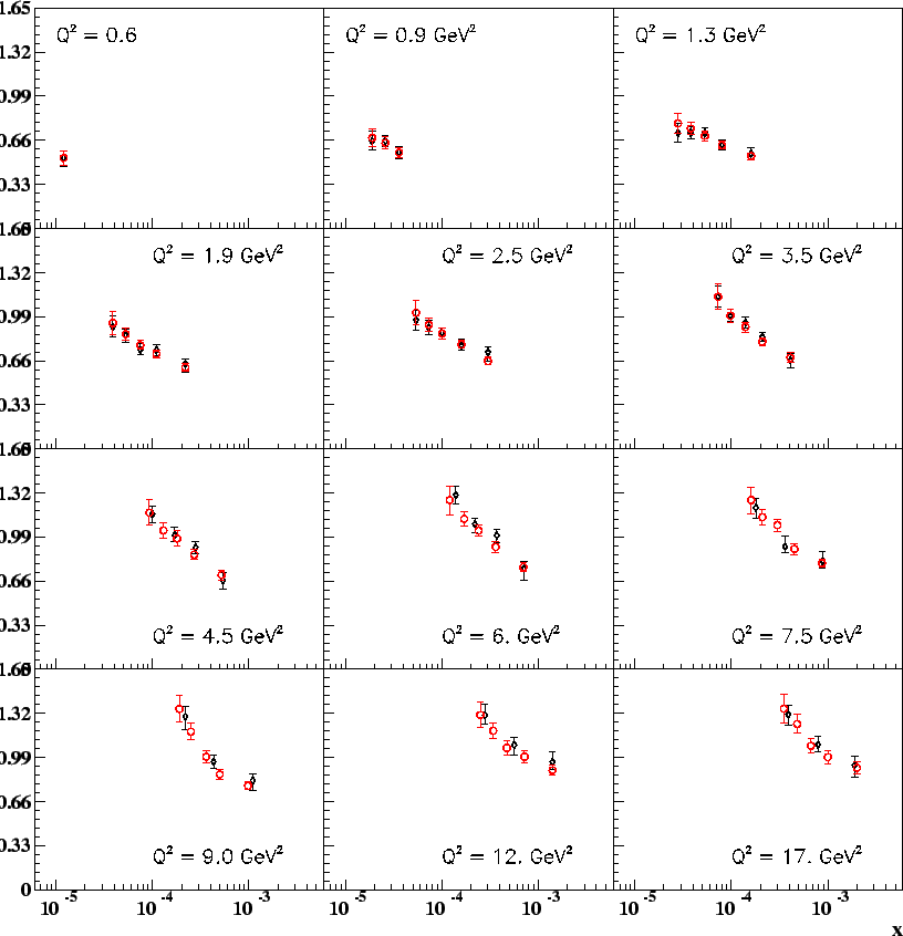$\begin{figure} \centerline{ \epsfig{figure=figure/f2_xt.eps,height=20cm,clip=}} \end{figure}$

Next: Bibliography Up: An update of the Previous: Conclusions

Giulio D'Agostini 2004-05-05