Next: Linear fit with normal
Up: Fits, and especially linear
Previous: Introduction
Probabilistic parametric inference from a set of
data points with errors on both axes
Let us consider a `law' that relates the `true' values of two
quantities, indicated here by
 and
and  :
:
 |
(3) |
where
 stands for the parameters
of the law, whose number is
stands for the parameters
of the law, whose number is  .
In the linear case Eq. (3) reduces to
.
In the linear case Eq. (3) reduces to
i.e.
 and
and  .
As it is well understood, because of `errors'
we do not observe directly and ,
but experimental quantities2
.
As it is well understood, because of `errors'
we do not observe directly and ,
but experimental quantities2
 and
and  that might differ,
on an event by event basis,
from and . The outcome of
the `observation' (see footnote 2)
that might differ,
on an event by event basis,
from and . The outcome of
the `observation' (see footnote 2)
 for a given
  (analogous reasonings
apply to
(analogous reasonings
apply to  and
and  )
is modeled by
an error function
)
is modeled by
an error function
 , that is indeed
a probability density function (pdf) conditioned by
and the `general state of knowledge'
, that is indeed
a probability density function (pdf) conditioned by
and the `general state of knowledge'  .
The latter stands for all background knowledge behind the analysis,
that is what for example makes us to believe
the relation
.
The latter stands for all background knowledge behind the analysis,
that is what for example makes us to believe
the relation
 ,
the particular mathematical expressions
for
and
,
the particular mathematical expressions
for
and
 ,
and so on. Note that
the shape of the error function might depend on the value of
,
as it happens if the detector does not respond the same way
to different solicitations.
A usual assumption is that
errors are normally distributed, i.e.
,
and so on. Note that
the shape of the error function might depend on the value of
,
as it happens if the detector does not respond the same way
to different solicitations.
A usual assumption is that
errors are normally distributed, i.e.
where the symbol ` ' stands for `is described by the distribution'
(or `follows the distribution'),
and where we still leave the possibility that the standard deviations,
that we consider known,
might be different in different observations.
Anyway, for sake of generality, we shall make use of
assumptions (5) and (6)
only in next section.
' stands for `is described by the distribution'
(or `follows the distribution'),
and where we still leave the possibility that the standard deviations,
that we consider known,
might be different in different observations.
Anyway, for sake of generality, we shall make use of
assumptions (5) and (6)
only in next section.
If we think of  pairs of measurements of and ,
before doing the experiment we are uncertain about
pairs of measurements of and ,
before doing the experiment we are uncertain about  quantities
(all 's, all 's, all 's and all 's, indicated respectively
as
quantities
(all 's, all 's, all 's and all 's, indicated respectively
as
 ,
,
 ,
,
 and
and
 )
plus the number of parameters, i.e. in total
)
plus the number of parameters, i.e. in total
 , that become
  in linear fits. [But note that, due to believed deterministic
relationship (3), the number of independent variables
is in fact
in linear fits. [But note that, due to believed deterministic
relationship (3), the number of independent variables
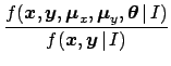
is in fact  .] Our final goal,
expressed in probabilistic terms, is to get the pdf
of the parameters given the experimental information
and all background knowledge:
.] Our final goal,
expressed in probabilistic terms, is to get the pdf
of the parameters given the experimental information
and all background knowledge:
Probability theory teaches us how to get
the conditional pdf
 if we know the joint distribution
 .
The first step consists in calculating the
.
The first step consists in calculating the  variable pdf
(only
variable pdf
(only  of which are independent)
that describes the uncertainty of what is not precisely known, given what
it is (plus all background knowledge). This is achieved
by a multivariate extension of Eq. (1):
of which are independent)
that describes the uncertainty of what is not precisely known, given what
it is (plus all background knowledge). This is achieved
by a multivariate extension of Eq. (1):
Equations (7) and (8) are two different
ways of writing Bayes' theorem in the case of multiple inference.
Going from (7) to (8) we have `marginalized'
over
,
and
, i.e.
we used an extension of
Eq. (2) to many variables.
[The standard text book version of the Bayes formula differs from
Eqs. (7) and (8) because the joint
pdf's that appear on the r.h.s. of Eqs. (7)-(8)
are usually factorized using the so called
'chain rule', i.e. an extension of Eq. (1)
to many variables.]
The second step consists in
marginalizing the  -dimensional pdf over the variables
we are not interested to:
-dimensional pdf over the variables
we are not interested to:
Before doing that, we note that the denominator of the r.h.s.
of Eqs. (7)-(8) is
just a number, once the model and the
set of observations
 is defined, and then we can
absorb it in the normalization constant.
Therefore Eq. (9) can be simply rewritten as
is defined, and then we can
absorb it in the normalization constant.
Therefore Eq. (9) can be simply rewritten as
We understand then that, essentially, we need to set up
using the pieces of information that come from our
background knowledge .
This seems a horrible task, but it becomes feasible tanks to
the chain rule of probability theory, that allows us to rewrite
in the following way:
(Obviously, among the several possible ones, we choose the factorization
that matches our knowledge about of physics case.)
At this point let us make the inventory of the ingredients,
stressing their effective conditions
and making use of independence, when it holds.
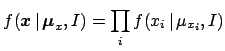
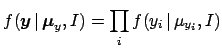
- Each observation depends directly only on the corresponding true value
:
(In square brackets is the `routinely' used pdf.)
- Each observation depends directly only on the corresponding true value
:
- Each true value depends only, and in a deterministic way,
on the corresponding true value
and on the parameters
. This is
formally equivalent to take an infinitely sharp distribution of
around
 ,
i.e. a Dirac delta function:
,
i.e. a Dirac delta function:
- Finally, and
are usually independent and
become the priors of the
problem,3
that one takes `vague' enough, unless physical motivations suggest to do
otherwise. For the we take immediately uniform distributions
over a large domain (a `flat prior').
Instead, we leave here the expression of
 undefined,
as a reminder for critical problems (e.g. one of the parameter is positively
defined because of its physical meaning),
though it can also be taken flat in routine
applications with `many' data points.
undefined,
as a reminder for critical problems (e.g. one of the parameter is positively
defined because of its physical meaning),
though it can also be taken flat in routine
applications with `many' data points.
The constant value of
 ,
indicated here by
,
indicated here by  ,
is then in practice absorbed in the normalization constant.
,
is then in practice absorbed in the normalization constant.
In conclusion we have
Figure 1:
Graphical representation of the model in term of a
Bayesian network (see text).
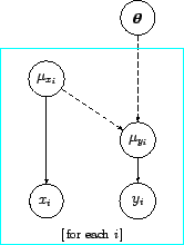 |
Figure 1
provides a graphical representation of
the model [or, more precisely, a
graphical representation of Eq. (20)].
In this diagram the probabilistic connections are indicated
by solid lines and the deterministic connections by
dashed lines.
These kind of networks of probabilistic and deterministic
relations among uncertain quantities is known as
`Bayesian network',4
'belief network', 'influence network', 'causal network'
and other names meaning substantially the same
thing.
From Eqs. (10) and (22) we get then
where we have factorized the unnormalized `final' pdf into the
`likelihood'5
 (the content of the large square bracket) and the `prior'
.
(the content of the large square bracket) and the `prior'
.
We see than that, a part from the prior, the result is essentially
given by the product of terms, each
of which depending on the individual pair of measurements:
where
and the constant factor  , irrelevant in the Bayes formula,
is a reminder of the priors about (see footnote 5).
, irrelevant in the Bayes formula,
is a reminder of the priors about (see footnote 5).
Next: Linear fit with normal
Up: Fits, and especially linear
Previous: Introduction
Giulio D'Agostini
2005-11-21
![$\displaystyle [\ \Longrightarrow \prod_i {\cal N}(\mu_{x_i},\sigma_{x_i}) \ ].$](img67.png)
![$\displaystyle [\ \Longrightarrow \prod_i {\cal N}(\mu_{y_i},\sigma_{y_i}) \ ].$](img70.png)
![$\displaystyle \prod_i \delta[\,\mu_{y_i}- \mu_{y}(\mu_{x_i},{\mbox{\boldmath$\theta$}})\,]$](img73.png)
![$\displaystyle [\ \Longrightarrow \prod_i \delta( \mu_{y_i} -m\, \mu_{x_i} - c )\ ]$](img74.png)
![$\displaystyle \prod_i f(x_i\,\vert\,\mu_{x_i},I) \cdot f(y_i\,\vert\,\mu_{y_i},...
...\,]\,
\cdot f(\mu_{x_i}\,\vert\,I)\cdot f({\mbox{\boldmath$\theta$}}\,\vert\,I)$](img81.png)
![$\displaystyle \prod_i k_{x_i}\,f(x_i\,\vert\,\mu_{x_i},I) \cdot f(y_i\,\vert\,\...
...,{\mbox{\boldmath$\theta$}})\,]\,
\cdot f({\mbox{\boldmath$\theta$}}\,\vert\,I)$](img82.png)
![$\displaystyle \prod_i f(x_i\,\vert\,\mu_{x_i},I) \cdot f(y_i\,\vert\,\mu_{y_i},...
...box{\boldmath$\theta$}})\,]\,
\cdot f({\mbox{\boldmath$\theta$}}\,\vert\,I) \,.$](img83.png)
![$\displaystyle \left[\int
\prod_i k_{x_i}\,f(x_i\,\vert\,\mu_{x_i},I) \cdot f(y_...
...{\mbox{\boldmath$\mu$}}_y \right]
\cdot f({\mbox{\boldmath$\theta$}}\,\vert\,I)$](img85.png)
![$\displaystyle \left[\prod_i {\cal L}_i({\mbox{\boldmath$\theta$}}\,;\,x_i,y_i,I)\right]
\cdot f({\mbox{\boldmath$\theta$}}\,\vert\,I)\,,$](img96.png)
![$\displaystyle k_{x_i}\, \int f(x_i\,\vert\,\mu_{x_i},I) \cdot f(y_i\,\vert\,\mu...
... \mu_{y}(\mu_{x_i},{\mbox{\boldmath$\theta$}})\,] \,\,
d{\mu_{x_i}}d{\mu_{y_i}}$](img98.png)