Systematic errors

Let us now consider the effect of systematic errors, i.e. errors that acts the same way on all observations of the sample, for example an uncertain offset in the instrument scale, or an uncertain scale factor. I do not want to give a complete treatment of the subjects, but focus only on how our systematic effects modify our graphical model, and give some practical rules for the simple case of linear fits. (For an introduction about systematic errors and their consistent treatment within the Bayesian approach see Ref. [2].)

For each coordinate we can introduce the fictitious quantities $\mu_x^S$ and $\mu_y^S$ that take into account the modification of $\mu_x$ and $\mu_y$ due to the systematic effect. For example, if the systematic effects only acts as an offset, i.e. we are uncertain about the `true' zero of the instruments, $\zeta_x$ and $\zeta_y$, we have

$$\mu_{x_i}^S = \mu_{x_i} + \zeta_x$$ (71)

$$\mu_{y_i}^S = \mu_{y_i} + \zeta_y\,,$$ (72)

where the true value of $\zeta_x$ are $\zeta_y$ unknown (otherwise there would be no systematic errors). We only know that their expected value is zero (otherwise we need to apply a calibration constant to the measurements) and we quantify our uncertainty with pdf's. For example, we could model them with Gaussian distributions:

$$\zeta_x \sim {\cal N}(0, \sigma_{\zeta_x})$$ (73)

$$\zeta_y \sim {\cal N}(0, \sigma_{\zeta_y})\,.$$ (74)

Anyway, for sake of generality, we leave the systematic effects in the most general form, dependent on the uncertain quantities ${\mbox{\boldmath$\beta$}}_x$ and ${\mbox{\boldmath$\beta$}}_y$ [to be clear: in the case of solely offset systematics we have ${\mbox{\boldmath$\beta$}}_x=\{\zeta_x\}$ ${\mbox{\boldmath$\beta$}}_y=\{\zeta_y\}$]. The values of $\mu_{x_i}^S$ and $\mu_{y_i}^S$ are modeled as follow

$$\mu_{x_i}^S \,: \ \ \mu_{x_i}^S \leftarrow \mu_{x}^S(\mu_{x_i};{\mbox{\boldmath$\beta$}}_x)$$ (75)

$$\mu_{y_i}^S \,: \ \ \mu_{y_i}^S \leftarrow \mu_{y}^S(\mu_{y_i};{\mbox{\boldmath$\beta$}}_y)$$ (76)

$${\mbox{\boldmath$\beta$}}_x \, : \ \ {\mbox{\boldmath$\beta$}}_x \sim f({\mbox{\boldmath$\beta$}}_x\,\vert\,I)$$ (77)

$${\mbox{\boldmath$\beta$}}_y \,: \ \ {\mbox{\boldmath$\beta$}}_y \sim f({\mbox{\boldmath$\beta$}}_y\,\vert\,I)\,.$$ (78)

Figure 3

Figure 3: Graphical model of Fig. 2 with the addition of systematic errors on both axes.

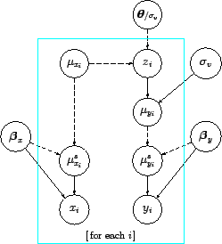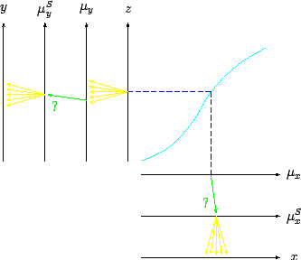
Figure 4: A different visual representation of the probabilistic model of Fig. 3.

shows the graphical model containing the new ingredients. The links ${\mbox{\boldmath$\beta$}}_x \rightarrow x_i$ and ${\mbox{\boldmath$\beta$}}_y \rightarrow y_i$ are to remember that systematics could also effect the error functions. An alternative visual picture of the probabilistic model is shown in Fig. 4. Note the different symbols to indicate the different uncertain processes: the divergent arrows (in yellow, if you are reading an electronic version of the paper) indicate that, given a value of the `parent' variable, the `child' variable fluctuates on an event-by-event basis; the green single arrow with the question mark indicate that, given a value of the `parent', the child will always take a fixed value, though we do not know which one.

Obviously, the practical implementation of complicate systematic effects in complicate fits can be quite challenging, but at least the Bayesian network provides an overall picture of the model. The simplest case is that of linear fit where only offset and scale uncertainty are present, with uncertainty modeled by a Gaussian distribution. This means that the ${\mbox{\boldmath$\beta$}}$'s and their uncertainty are as follows ($\eta$ is the scale factor of uncertain value):

$${\mbox{\boldmath$\beta$}}_x = \{\zeta_x,\eta_x\} \hspace{3.0mm} \hspace{3.0mm} {\mbox{\boldmath$\beta$}}_y = \{\zeta_y,\eta_y\}$$ (79)

$$\zeta_x \sim {\cal N}(0,\sigma_{\zeta_x}) \hspace{3.0mm} \hspace{3.0mm}\zeta_y \sim {\cal N}(0,\sigma_{\zeta_y})$$ (80)

$$\eta_x \sim {\cal N}(1,\sigma_{\eta_x}) \hspace{3.0mm} \hspace{3.0mm}\eta_y \sim {\cal N}(1,\sigma_{\eta_y})$$ (81)

In this case we can get an hint of how the uncertainty about $m$ and $c$ change without doing the full calculation following an heuristic approach, valid when $f(m,c)$ is approximately multivariate Gaussian and the details of which can be found in Ref. [16]. We obtain the following results, in which $\left.\sigma(m)\right\vert _{\zeta_x}$ indicates the contribution to the uncertainty about the slope $m$ due to uncertainty about $\zeta_x$, $\left.\sigma(m)\right\vert _{\eta_x}$ that due to the scale factor $\eta_x$, and so on⁷:

$$\left.\sigma(m)\right\vert _{\zeta_x} = 0$$ (82)

$$\left.\sigma(m)\right\vert _{\zeta_y} = 0$$ (83)

$$\left.\sigma(c)\right\vert _{\zeta_x} = \vert m\vert\,\sigma_{\zeta_x}$$ (84)

$$\left.\sigma(c)\right\vert _{\zeta_y} = \sigma_{\zeta_y}$$ (85)

$$\left.\sigma(m)\right\vert _{\eta_x} = \vert m\vert\,\sigma_{\eta_x}$$ (86)

$$\left.\sigma(m)\right\vert _{\eta_y} = \vert m\vert\,\sigma_{\eta_y}$$ (87)

$$\left.\sigma(c)\right\vert _{\eta_x} = 0$$ (88)

$$\left.\sigma(c)\right\vert _{\eta_y} = \vert c\vert\,\sigma_{\eta_y} \,.$$ (89)

All contributions are then added quadratically to the so called `statistical' ones.