Next: Partial results from ,
Up: Inferring and of the
Previous: Introduction
Uncertain constraints
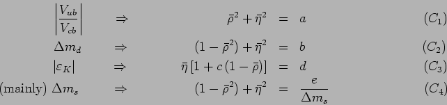
The relations (1)-(4) of Ref. [1] can be written
in the following way
where  ,
, , ...
, ... are the constraint parameters, functions
of many quantities; the most crucial of those determined experimentally
are indicated on the left hand side of the equations.
Note that the order of
are the constraint parameters, functions
of many quantities; the most crucial of those determined experimentally
are indicated on the left hand side of the equations.
Note that the order of  and
and  is exchanged with respect to
Eqs. (3)-(4) of Ref. [1]. This is because,
since the present information concerning
is exchanged with respect to
Eqs. (3)-(4) of Ref. [1]. This is because,
since the present information concerning  is of different quality with respect to the other quantities,
the constraint needs a more careful treatment than the others,
and it will be introduced after
is of different quality with respect to the other quantities,
the constraint needs a more careful treatment than the others,
and it will be introduced after  -.
This is also the reason why appears explicitly in
the constraint .
-.
This is also the reason why appears explicitly in
the constraint .
In the ideal case all parameters are perfectly known,
and the constraints would give curves in the  -
- plane.
For example, would give a circle of radius
plane.
For example, would give a circle of radius  .
In other terms, due to this constraint all
points of the circumference would be appear to us likely,
unless
there is any other experimental piece of information
(or theoretical prejudice) to assign a different weight to
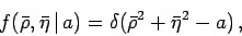
different points. In the ideal case
the p.d.f. describing our beliefs
in the and values would be
.
In other terms, due to this constraint all
points of the circumference would be appear to us likely,
unless
there is any other experimental piece of information
(or theoretical prejudice) to assign a different weight to
different points. In the ideal case
the p.d.f. describing our beliefs
in the and values would be
 |
(1) |
with the Dirac delta meaning the limit
of a very narrow p.d.f. concentrated on the circumference.
Similar arguments hold for the parameters of the
other constraints. Let us call them generically  (the fact that depends on two parameters is conceptually
irrelevant).
(the fact that depends on two parameters is conceptually
irrelevant).
In the real case itself is not perfectly known.
There are values which are more likely, and values
which are less likely, classified
by the p.d.f.  . This means that, e.g. for the parameter ,
we deal with an infinite number
of circles, each having its weight
. This means that, e.g. for the parameter ,
we deal with an infinite number
of circles, each having its weight  . It follows that the points
of the (, ) plane get different weights.
. It follows that the points
of the (, ) plane get different weights.
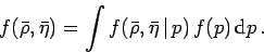
The probability theory teaches us how to evaluate
 taking into account all possible values of :
 |
(2) |
Now the problem becomes how to evaluate , knowing that
each depends on many input quantities  ,
denoted all together with
,
denoted all together with
 and described, in the most general case,
by a joint p.d.f.
and described, in the most general case,
by a joint p.d.f.  .
In most
cases of practical interest, including the one we are discussing,
each can be considered independent from the others,
and the joint distribution simplifies to
.
In most
cases of practical interest, including the one we are discussing,
each can be considered independent from the others,
and the joint distribution simplifies to
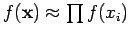 . Calling
  the function
which relates to , can be generally
obtained as
the function
which relates to , can be generally
obtained as
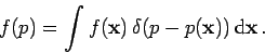 |
(3) |
This integral, as well as the previous integrals, is usually performed
by Monte Carlo techniques.
The calculations can be simplified in the following way.
- First, we rely on the central limit theorem, assuming
to be Gaussian
for all parameters (but with no constraint on the shape of
!).
- Expected value, standard (deviation) uncertainty and correlation
are basically obtained by the usual propagation (see Ref. [5]
for a similar application).
- Non linear effects in the propagation have been taken into
account up to second order, using formulae of Ref. [6]
(see this paper for the practical modeling of uncertainties and
treatment of asymmetric cases).
- The correlation between
 and
and  has been taken into account
building a bi-variate
has been taken into account
building a bi-variate  .
.
As input quantities, Table 1 of Ref. [1] is used, combining
properly (i.e. quadratically) the standard deviations.
For example, for
 expressed in MeV we obtain
 , where
 stands for the standard deviation
of a uniform distribution of half width 20 MeV.
Note that, contrary to what some authors critical
about Ref. [1] (and the related papers and presentations
to conferences) think, I have the impression that my colleagues
tend to make slightly conservative assessments
of uncertainties. This feeling that I had a priori
discussing with them is somewhat confirmed
a posteriori by the excellent overlap of the partial
inference by each constraint (as it will be shown in
Fig. 9) and self-consistency
between input parameters and values coming out of
the inference obtained without the their contribution
(see Ref. [1]).
stands for the standard deviation
of a uniform distribution of half width 20 MeV.
Note that, contrary to what some authors critical
about Ref. [1] (and the related papers and presentations
to conferences) think, I have the impression that my colleagues
tend to make slightly conservative assessments
of uncertainties. This feeling that I had a priori
discussing with them is somewhat confirmed
a posteriori by the excellent overlap of the partial
inference by each constraint (as it will be shown in
Fig. 9) and self-consistency
between input parameters and values coming out of
the inference obtained without the their contribution
(see Ref. [1]).
The following results are obtained in terms of expected values and
standard deviations (``
 ''):
''):
Only the correlation between and is relevant, and all
others can be neglected, being below the 10% level
(even that between and , related by  , is negligible,
being only +7%). The radii of the circles given by
and
, is negligible,
being only +7%). The radii of the circles given by
and  are
are  and
and  , respectively.
These radii have the meaning of the sides of the unitarity triangle opposite
to
, respectively.
These radii have the meaning of the sides of the unitarity triangle opposite
to  and
and  , respectively, provided
by and alone.
, respectively, provided
by and alone.
Next: Partial results from ,
Up: Inferring and of the
Previous: Introduction
Giulio D'Agostini
2004-01-20