Foreword
These slides are a notebook converted to (HTML) slides via the jupyter-nbconvert utility.
Get the code from gitlab here: https://gitlab.com/carlomt/pycourse with, in an new terminal:
git clone https://gitlab.com/carlomt/pycourse
cd pycourse
conda env create -f environment.yml
conda activate pycourse
. post-install.sh #Configure some extra stuff
The pre-installed environment course is enough to read/edit these slides.
Read the README.md file for additional instructions.
Python Perugia INFN Course: Data Science tools
This material is available on gitlab
Contact us: andrea.dotti@gmail.com, mancinit@infn.it
The SciPy library contains several packages to perform specialized scientific calculations:
- Special functions (
scipy.special) - Integration (
scipy.integrate) - Optimization (
scipy.optimize) - Interpolation (
scipy.interpolate) - Fourier Transforms (
scipy.fftpack) - Signal Processing (
scipy.signal) - Linear Algebra (
scipy.linalg) - Sparse Eigenvalue Problems with ARPACK
- Compressed Sparse Graph Routines (
scipy.sparse.csgraph) - Spatial data structures and algorithms (
scipy.spatial) - Statistics (
scipy.stats) - Multidimensional image processing (
scipy.ndimage) - File IO (
scipy.io)
![]()
Numpy
It is the foundation of python scientific stack.
The basic building block is the numpy.array data structure. It can be used as a python list of numbers, but it is a specialized efficient way of manipulating numbers in python.
import numpy as np
a = np.array([1, 2, 3, 4], dtype=float)
a
array([1., 2., 3., 4.])
a = range(1000)
%timeit [ i**2 for i in a]
280 µs ± 8.64 µs per loop (mean ± std. dev. of 7 runs, 1000 loops each)
b = np.arange(1000)
%timeit b**2
1.02 µs ± 45.7 ns per loop (mean ± std. dev. of 7 runs, 1000000 loops each)
c = np.array([[1,2],[3,4]])
c
array([[1, 2],
       [3, 4]])
c.ndim
2
c.shape
(2, 2)
c = np.arange(27)
c.reshape((3,3,3))
array([[[ 0,  1,  2],
        [ 3,  4,  5],
        [ 6,  7,  8]],

       [[ 9, 10, 11],
        [12, 13, 14],
        [15, 16, 17]],

       [[18, 19, 20],
        [21, 22, 23],
        [24, 25, 26]]])
np.zeros((2,2))
array([[0., 0.],
       [0., 0.]])
np.ones((2,1))
array([[1.],
       [1.]])
a = np.arange(27).reshape((3,3,3))
np.ones_like(a)
array([[[1, 1, 1],
        [1, 1, 1],
        [1, 1, 1]],

       [[1, 1, 1],
        [1, 1, 1],
        [1, 1, 1]],

       [[1, 1, 1],
        [1, 1, 1],
        [1, 1, 1]]])
np.eye(3)
array([[1., 0., 0.],
       [0., 1., 0.],
       [0., 0., 1.]])
a = np.arange(10)
a
array([0, 1, 2, 3, 4, 5, 6, 7, 8, 9])
a[0]
0
a[-1]
9
a[0:3]
array([0, 1, 2])
a[::2]
array([0, 2, 4, 6, 8])
a = a.reshape(5,2)
a
array([[0, 1],
       [2, 3],
       [4, 5],
       [6, 7],
       [8, 9]])
a[3,1]
7
a[2,:]
array([4, 5])
Important: Views or copy
A slice or reshape is a view, simply a re-organization of the same data in memory, thus changing one element changes the same element in all views
a = np.arange(9)
b = a.reshape((3,3))
np.shares_memory(a,b)
True
a[3] = -1
b
array([[ 0,  1,  2],
       [-1,  4,  5],
       [ 6,  7,  8]])
np.shares_memory(a,b)
True
b = a.copy()
np.shares_memory(a,b)
False
Boolean masks for extracting values
A typical operation done in your daily physics data analysis is to extract from an array the values that match a condition. Consider an array of the energies of particles, and assume you want to use only the energies above a given threshold. Boolean masking comes at a rescue
ene = np.random.exponential(size=10, scale=10.) # 1/scale e^(-ene/scale)
ene
array([26.78949043, 39.75183681,  0.36677236,  3.8809366 ,  0.54143778,
        3.64373788, 44.26306009,  0.63227985, 16.09218254,  5.13612747])
mask = ene > 2
mask
array([ True,  True, False,  True, False,  True,  True, False,  True,
        True])
ene[mask]
array([26.78949043, 39.75183681,  3.8809366 ,  3.64373788, 44.26306009,
       16.09218254,  5.13612747])
ene[ene<2]
array([0.36677236, 0.54143778, 0.63227985])
ene[ene<2] = 0
ene
array([26.78949043, 39.75183681,  0.        ,  3.8809366 ,  0.        ,
        3.64373788, 44.26306009,  0.        , 16.09218254,  5.13612747])
Values with list of indexes
Similarly to boolean masks, it is possible to access and modify values directly to an array using a list of indexes
status = np.random.randint(low=0,high=10,size=10)
status
array([3, 1, 3, 2, 1, 2, 8, 5, 7, 4])
status[[0, 3, 5]]
array([3, 2, 2])
status[[0, 3, 5]] = -1
status
array([-1, 1, 3, -1, 1, -1, 8, 5, 7, 4])
Simple Operations
a = np.arange(4)
a
array([0, 1, 2, 3])
a+1
array([1, 2, 3, 4])
10**a
array([ 1, 10, 100, 1000])
np.sin(a)
array([0. , 0.84147098, 0.90929743, 0.14112001])
Reductions
a = np.random.randint(low=0,high=10,size=4)
a
array([2, 8, 7, 7])
np.sum(a)
24
np.max(a), np.min(a)
(8, 2)
np.argmax(a), np.argmin(a)
(1, 0)
np.mean(a), np.median(a), np.std(a)
(6.0, 7.0, 2.345207879911715)
a = a.reshape(2,2)
a
array([[2, 8],
       [7, 7]])
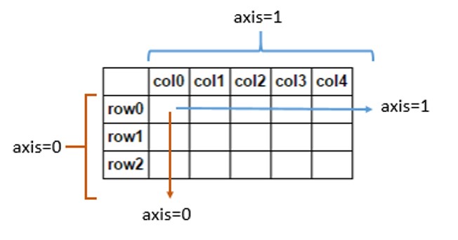
np.sum(a,axis=1)
array([10, 14])
m1 = a>3
m1
array([[False,  True],
       [ True,  True]])
np.all(m1)
False
np.any(m1)
True
Matplotlib
Matplotlib is probably the most used Python package for 2D-graphics. It provides both a quick way to visualize data from Python and publication-quality figures in many formats.
Other visualization packages exists, often these are built on top of matplotlib.
The package is well integrated into IPython and Jupyter.
%matplotlib inline
from matplotlib import pyplot as plt
import numpy as np
X = np.linspace(-np.pi, np.pi, 256, endpoint=True)
C, S = np.cos(X), np.sin(X)
plt.plot(X,C)
plt.plot(X,S)
[<matplotlib.lines.Line2D at 0x7fbd7c35f810>]

Customization
plt.figure(figsize=(4, 3), dpi=80)
plt.plot(X, C, color="blue", linewidth=1.0, linestyle="-", label="cos")
plt.plot(X, S, color="green", linewidth=1.0, linestyle="-", label="sin")
plt.xlim(-4.0, 4.0)
plt.xticks(np.linspace(-4, 4, 9, endpoint=True))
plt.savefig("example.png", dpi=72)
plt.grid()
plt.xlabel("x")
plt.ylabel("y")
plt.title("Example")
plt.legend(loc="best")
<matplotlib.legend.Legend at 0x7fbd7c2d1850>

Multiple plots
plt.figure(figsize=(6, 4))
plt.subplot(2, 2, 1)
plt.plot(X, C, color="blue", linewidth=1.0, linestyle="-", label="cos")
plt.subplot(2, 2, 2)
plt.plot(X, S, color="green", linewidth=1.0, linestyle="-", label="sin")
plt.subplot(2, 2, 3)
plt.plot(X, C, color="red", linewidth=1.0, linestyle="-", label="cos")
plt.subplot(2, 2, 4)
plt.plot(X, S, color="black", linewidth=1.0, linestyle="-", label="sin")
plt.show()

Examples
plt.rcdefaults()
fig, ax = plt.subplots(figsize=(4,3))
# Example data
people = ('Tom', 'Dick', 'Harry', 'Slim', 'Jim')
y_pos = np.arange(len(people))
performance = 3 + 10 * np.random.rand(len(people))
error = np.random.rand(len(people))
ax.barh(y_pos, performance, xerr=error, align='center',
        color='green', ecolor='black')
ax.set_yticks(y_pos)
ax.set_yticklabels(people)
ax.invert_yaxis()  # labels read top-to-bottom
ax.set_xlabel('Performance')
ax.set_title('How fast do you want to go today?')

plt.show()

x = np.linspace(0, 1, 500)
y = np.sin(4 * np.pi * x) * np.exp(-5 * x)
fig, ax = plt.subplots()
ax.fill(x, y, zorder=10)
ax.grid(True, zorder=5)
plt.show()

fig, ax = plt.subplots()
for color in ['red', 'green', 'blue']:
    n = 750
    x, y = np.random.rand(2, n)
    scale = 200.0 * np.random.rand(n)
    ax.scatter(x, y, c=color, s=scale, label=color,
               alpha=0.3, edgecolors='none')

ax.legend()
ax.grid(True)

plt.show()

mu = 200
sigma = 25
x = np.random.normal(mu, sigma, size=100)
fig, (ax0, ax1) = plt.subplots(ncols=2, figsize=(6, 3))
ax0.hist(x, 20, density=1, histtype='stepfilled', facecolor='g', alpha=0.75)
ax0.set_title('stepfilled')
# Create a histogram by providing the bin edges (unequally spaced).
bins = [100, 150, 180, 195, 205, 220, 250, 300]
ax1.hist(x, bins, density=1, histtype='bar', rwidth=0.8)
ax1.set_title('unequal bins')
plt.title(r'Histogram of IQ: $\mu=100$, $\sigma=15$');

from matplotlib import colors, ticker, cm
from scipy.stats import multivariate_normal

N = 100
x = np.linspace(-3.0, 3.0, N)
y = np.linspace(-2.0, 2.0, N)

X, Y = np.meshgrid(x, y)
pos = np.empty(X.shape+(2,))
pos[:,:,0] = X; pos[:,:,1] = Y
# A low hump with a spike coming out of the top right.
# Needs to have z/colour axis on a log scale so we see both hump and spike.
# linear scale only shows the spike.
z = (multivariate_normal([0.1, 0.2], [[1.0, 0.],[0, 1.0]]).pdf(pos)
     + 0.1 * (multivariate_normal([1.0, 1.0],[[0.01, 0.],[0., 0.01]])).pdf(pos))
# Automatic selection of levels works; setting the
# log locator tells contourf to use a log scale:
fig, ax = plt.subplots(figsize=(4,3))
cs = ax.contourf(X, Y, z, locator=ticker.LogLocator(), cmap=cm.PuBu_r)
cbar = fig.colorbar(cs)

![]()
Pandas
Pandas is a high-performance, high-level library that provides tools for data analysis.
It relies on the concept of DataFrame: a structured collection of data organized in records. This is the same concept of ROOT's NTuple that you are familiar with.
I think the name comes from R.
import numpy as np
import pandas as pd

s = pd.Series( [1., 2., 3., np.nan, 5. ], index=["a","b","c","d","e"])
s
a    1.0
b    2.0
c    3.0
d    NaN
e    5.0
dtype: float64
df = pd.DataFrame(
    {
        'Col1': [1.,2.,3.,4.],
        'Col2': ["a","b","c","d"],
        'Col3': [True, False, True, True]
    }
)
df
| Col1 | Col2 | Col3 | |
|---|---|---|---|
| 0 | 1.0 | a | True |
| 1 | 2.0 | b | False |
| 2 | 3.0 | c | True |
| 3 | 4.0 | d | True |
Reading/Saving dataframes
Pandas support reading writing to several data formats, via specialized routines, many other formats, because dataframe (with other names) are a common concept:
| Format Type | Data Description | Reader | Writer |
|---|---|---|---|
| text | CSV | read_csv |
to_csv |
| text | JSON | read_json |
to_json |
| text | HTML | read_html |
to_html |
| text | Local clipboard | read_clipboard |
to_clipboard |
| binary | MS Excel | read_excel |
to_excel |
| binary | HDF5 Format | read_hdf |
to_hdf |
| binary | Feather Format | read_feather |
to_feather |
| binary | Parquet Format | read_parquet |
to_parquet |
| binary | Msgpack | read_msgpack |
to_msgpack |
| binary | Stata | read_stata |
to_stata |
| binary | SAS | read_sas |
|
| binary | Pickle Format | read_pickle |
to_pickle |
| SQL | SQL | read_sql |
to_sql |
| SQL | Google Big Query | read_gbq |
to_gbq |
As you can see the physicists ROOT format is not natively supported. However some external software to read TTrees are available. For example root_numpy, root_pandas, or uproot. ROOT usually comes with pre-installed pyROOT library (the one on the provided VM works only for python2), that offers basic functionalities.
df.dtypes
Col1    float64
Col2     object
Col3       bool
dtype: object
df.columns
Index(['Col1', 'Col2', 'Col3'], dtype='object')
df.index
RangeIndex(start=0, stop=4, step=1)
View data
df = pd.DataFrame( {'A':np.random.randint(0,10,100), 'B': [2**x for x in np.arange(100)], 'C':"a"})
df.head()
| A | B | C | |
|---|---|---|---|
| 0 | 9 | 1 | a |
| 1 | 9 | 2 | a |
| 2 | 9 | 4 | a |
| 3 | 0 | 8 | a |
| 4 | 3 | 16 | a |
df.tail(2)
| A | B | C | |
|---|---|---|---|
| 98 | 0 | 0 | a |
| 99 | 7 | 0 | a |
df.describe()
| A | B | |
|---|---|---|
| count | 100.000000 | 1.000000e+02 |
| mean | 4.150000 | -2.560000e+00 |
| std | 3.176222 | 1.070389e+18 |
| min | 0.000000 | -9.223372e+18 |
| 25% | 1.000000 | 0.000000e+00 |
| 50% | 4.000000 | 6.144000e+03 |
| 75% | 7.000000 | 1.717987e+11 |
| max | 9.000000 | 4.611686e+18 |
Select data
dates = pd.date_range('20190527',periods=7)
df = pd.DataFrame( np.random.rand(7,4), index=dates, columns=['A','B','C','D'])
df
| A | B | C | D | |
|---|---|---|---|---|
| 2019-05-27 | 0.272727 | 0.782185 | 0.871513 | 0.764663 |
| 2019-05-28 | 0.063530 | 0.615451 | 0.009551 | 0.969182 |
| 2019-05-29 | 0.635973 | 0.778371 | 0.927694 | 0.971305 |
| 2019-05-30 | 0.610504 | 0.943599 | 0.580770 | 0.994840 |
| 2019-05-31 | 0.738883 | 0.543482 | 0.686757 | 0.532077 |
| 2019-06-01 | 0.247118 | 0.453881 | 0.635333 | 0.659595 |
| 2019-06-02 | 0.215886 | 0.674861 | 0.180832 | 0.140780 |
df['A'] # or df.A
2019-05-27    0.272727
2019-05-28    0.063530
2019-05-29    0.635973
2019-05-30    0.610504
2019-05-31    0.738883
2019-06-01    0.247118
2019-06-02    0.215886
Freq: D, Name: A, dtype: float64
df[0:2]
| A | B | C | D | |
|---|---|---|---|---|
| 2019-05-27 | 0.272727 | 0.782185 | 0.871513 | 0.764663 |
| 2019-05-28 | 0.063530 | 0.615451 | 0.009551 | 0.969182 |
df['20190529':'20190531']
| A | B | C | D | |
|---|---|---|---|---|
| 2019-05-29 | 0.635973 | 0.778371 | 0.927694 | 0.971305 |
| 2019-05-30 | 0.610504 | 0.943599 | 0.580770 | 0.994840 |
| 2019-05-31 | 0.738883 | 0.543482 | 0.686757 | 0.532077 |
dates
DatetimeIndex(['2019-05-27', '2019-05-28', '2019-05-29', '2019-05-30',
               '2019-05-31', '2019-06-01', '2019-06-02'],
              dtype='datetime64[ns]', freq='D')
df.loc[dates[2]]
A    0.635973
B    0.778371
C    0.927694
D    0.971305
Name: 2019-05-29 00:00:00, dtype: float64
df.loc[dates[2],['B','C']]
B    0.778371
C    0.927694
Name: 2019-05-29 00:00:00, dtype: float64
df.iloc[2,1:3]
B    0.778371
C    0.927694
Name: 2019-05-29 00:00:00, dtype: float64
df[ df>0.5 ]
| A | B | C | D | |
|---|---|---|---|---|
| 2019-05-27 | NaN | 0.782185 | 0.871513 | 0.764663 |
| 2019-05-28 | NaN | 0.615451 | NaN | 0.969182 |
| 2019-05-29 | 0.635973 | 0.778371 | 0.927694 | 0.971305 |
| 2019-05-30 | 0.610504 | 0.943599 | 0.580770 | 0.994840 |
| 2019-05-31 | 0.738883 | 0.543482 | 0.686757 | 0.532077 |
| 2019-06-01 | NaN | NaN | 0.635333 | 0.659595 |
| 2019-06-02 | NaN | 0.674861 | NaN | NaN |
Setting values
s = pd.Series( np.random.rand(7), index=dates )
s
2019-05-27    0.084900
2019-05-28    0.337333
2019-05-29    0.465100
2019-05-30    0.517110
2019-05-31    0.688339
2019-06-01    0.455821
2019-06-02    0.907693
Freq: D, dtype: float64
df['E'] = s
df
| A | B | C | D | E | |
|---|---|---|---|---|---|
| 2019-05-27 | 0.272727 | 0.782185 | 0.871513 | 0.764663 | 0.084900 |
| 2019-05-28 | 0.063530 | 0.615451 | 0.009551 | 0.969182 | 0.337333 |
| 2019-05-29 | 0.635973 | 0.778371 | 0.927694 | 0.971305 | 0.465100 |
| 2019-05-30 | 0.610504 | 0.943599 | 0.580770 | 0.994840 | 0.517110 |
| 2019-05-31 | 0.738883 | 0.543482 | 0.686757 | 0.532077 | 0.688339 |
| 2019-06-01 | 0.247118 | 0.453881 | 0.635333 | 0.659595 | 0.455821 |
| 2019-06-02 | 0.215886 | 0.674861 | 0.180832 | 0.140780 | 0.907693 |
df.loc[:,['C']] = 0
df
| A | B | C | D | E | |
|---|---|---|---|---|---|
| 2019-05-27 | 0.272727 | 0.782185 | 0.0 | 0.764663 | 0.084900 |
| 2019-05-28 | 0.063530 | 0.615451 | 0.0 | 0.969182 | 0.337333 |
| 2019-05-29 | 0.635973 | 0.778371 | 0.0 | 0.971305 | 0.465100 |
| 2019-05-30 | 0.610504 | 0.943599 | 0.0 | 0.994840 | 0.517110 |
| 2019-05-31 | 0.738883 | 0.543482 | 0.0 | 0.532077 | 0.688339 |
| 2019-06-01 | 0.247118 | 0.453881 | 0.0 | 0.659595 | 0.455821 |
| 2019-06-02 | 0.215886 | 0.674861 | 0.0 | 0.140780 | 0.907693 |
Operations
df.mean()
A    0.397803
B    0.684547
C    0.000000
D    0.718920
E    0.493756
dtype: float64
df.mean(axis=1)
2019-05-27    0.380895
2019-05-28    0.397099
2019-05-29    0.570150
2019-05-30    0.613211
2019-05-31    0.500556
2019-06-01    0.363283
2019-06-02    0.387844
Freq: D, dtype: float64
Merging dataframes
df1 = pd.DataFrame( np.random.rand(7,2), index=dates, columns=['A','B'])
df2 = pd.DataFrame( np.random.rand(7,3), index=dates, columns=['C','D','E'])
pd.concat([df1,df2],sort=False)
| A | B | C | D | E | |
|---|---|---|---|---|---|
| 2019-05-27 | 0.933696 | 0.595231 | NaN | NaN | NaN |
| 2019-05-28 | 0.743323 | 0.174635 | NaN | NaN | NaN |
| 2019-05-29 | 0.534813 | 0.248670 | NaN | NaN | NaN |
| 2019-05-30 | 0.515590 | 0.645915 | NaN | NaN | NaN |
| 2019-05-31 | 0.034665 | 0.791540 | NaN | NaN | NaN |
| 2019-06-01 | 0.408191 | 0.827338 | NaN | NaN | NaN |
| 2019-06-02 | 0.333172 | 0.726970 | NaN | NaN | NaN |
| 2019-05-27 | NaN | NaN | 0.021164 | 0.856063 | 0.664016 |
| 2019-05-28 | NaN | NaN | 0.987556 | 0.649094 | 0.277106 |
| 2019-05-29 | NaN | NaN | 0.545813 | 0.103561 | 0.637652 |
| 2019-05-30 | NaN | NaN | 0.478624 | 0.849072 | 0.540173 |
| 2019-05-31 | NaN | NaN | 0.230484 | 0.758756 | 0.457617 |
| 2019-06-01 | NaN | NaN | 0.061748 | 0.648818 | 0.480178 |
| 2019-06-02 | NaN | NaN | 0.643230 | 0.200065 | 0.312921 |
pd.concat([df1,df2],axis=1,join='inner') #same syntax as for db (ineer, outer, left, right)
| A | B | C | D | E | |
|---|---|---|---|---|---|
| 2019-05-27 | 0.933696 | 0.595231 | 0.021164 | 0.856063 | 0.664016 |
| 2019-05-28 | 0.743323 | 0.174635 | 0.987556 | 0.649094 | 0.277106 |
| 2019-05-29 | 0.534813 | 0.248670 | 0.545813 | 0.103561 | 0.637652 |
| 2019-05-30 | 0.515590 | 0.645915 | 0.478624 | 0.849072 | 0.540173 |
| 2019-05-31 | 0.034665 | 0.791540 | 0.230484 | 0.758756 | 0.457617 |
| 2019-06-01 | 0.408191 | 0.827338 | 0.061748 | 0.648818 | 0.480178 |
| 2019-06-02 | 0.333172 | 0.726970 | 0.643230 | 0.200065 | 0.312921 |
Grouping
s = pd.Series( ["a","b","a","c","a","c","b"], index=dates)
df['E']=s
df
| A | B | C | D | E | |
|---|---|---|---|---|---|
| 2019-05-27 | 0.272727 | 0.782185 | 0.0 | 0.764663 | a |
| 2019-05-28 | 0.063530 | 0.615451 | 0.0 | 0.969182 | b |
| 2019-05-29 | 0.635973 | 0.778371 | 0.0 | 0.971305 | a |
| 2019-05-30 | 0.610504 | 0.943599 | 0.0 | 0.994840 | c |
| 2019-05-31 | 0.738883 | 0.543482 | 0.0 | 0.532077 | a |
| 2019-06-01 | 0.247118 | 0.453881 | 0.0 | 0.659595 | c |
| 2019-06-02 | 0.215886 | 0.674861 | 0.0 | 0.140780 | b |
df.groupby('E').sum()
| A | B | C | D | |
|---|---|---|---|---|
| E | ||||
| a | 1.647583 | 2.104038 | 0.0 | 2.268045 |
| b | 0.279415 | 1.290312 | 0.0 | 1.109962 |
| c | 0.857622 | 1.397480 | 0.0 | 1.654435 |
Pivot table
dates = pd.date_range('20190527',periods=6, name='date')
df = pd.DataFrame( np.random.rand(6,3), index=dates, columns=['A','B','C'])
df['D'] = pd.Series(["a","a","b","b","c","c"],index=dates)
df['E'] = pd.Series(["one","two","one","two","one","two"],index=dates)
df
| A | B | C | D | E | |
|---|---|---|---|---|---|
| date | |||||
| 2019-05-27 | 0.829799 | 0.720495 | 0.173438 | a | one |
| 2019-05-28 | 0.252488 | 0.014775 | 0.521227 | a | two |
| 2019-05-29 | 0.646422 | 0.112209 | 0.143434 | b | one |
| 2019-05-30 | 0.841273 | 0.665084 | 0.762137 | b | two |
| 2019-05-31 | 0.780462 | 0.595384 | 0.826812 | c | one |
| 2019-06-01 | 0.551363 | 0.768771 | 0.079635 | c | two |
pd.pivot_table(df, values=['A','B','C'], index=['D','E'])
| A | B | C | ||
|---|---|---|---|---|
| D | E | |||
| a | one | 0.829799 | 0.720495 | 0.173438 |
| two | 0.252488 | 0.014775 | 0.521227 | |
| b | one | 0.646422 | 0.112209 | 0.143434 |
| two | 0.841273 | 0.665084 | 0.762137 | |
| c | one | 0.780462 | 0.595384 | 0.826812 |
| two | 0.551363 | 0.768771 | 0.079635 |
Plotting data
%matplotlib inline
df.plot()
<AxesSubplot:xlabel='date'>
