Our a priori value of the mass is that it is positive
and not too large (otherwise it would already have been measured
in other experiments). One
can take any vague distribution which assigns a probability
density function between 0 and 20 or 30
eV .
In fact, if an experiment having a resolution of
.
In fact, if an experiment having a resolution of
 eV
has been planned and financed by rational people, with
the hope of finding evidence of non-negligible mass,
it means that the mass was thought to be in that range.
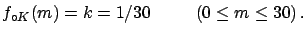
If there is no reason to prefer one of the values in that interval
a uniform distribution can be used, for example
eV
has been planned and financed by rational people, with
the hope of finding evidence of non-negligible mass,
it means that the mass was thought to be in that range.
If there is no reason to prefer one of the values in that interval
a uniform distribution can be used, for example
 |
(5.21) |
Otherwise, if one thinks
there is a greater chance of the mass having
small rather than high values,
a prior which reflects
such an assumption could be chosen,
for example a half normal with
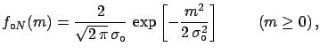
![$\displaystyle f_{\circ N}(m) =\frac{2}{\sqrt{2\,\pi}\,\sigma_\circ} \,\exp{\left[-\frac{m^2}{2\,\sigma_\circ^2}\right]} \hspace{1.0cm} (m \ge 0)\,,$](img687.png) |
(5.22) |
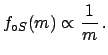
or a triangular distribution
 |
(5.23) |
Let us consider for simplicity the uniform distribution
The value which has the highest degree of belief is  ,
but
,
but  is non vanishing up to
 eV (even if very small).
We can define an interval, starting from ,
in which we believe that
eV (even if very small).
We can define an interval, starting from ,
in which we believe that  should have a certain
probability. For example
this level of probability can be
should have a certain
probability. For example
this level of probability can be  . One has to find the value
 for which the cumulative function
 equals 0.95.
This value of is called the upper limit (or upper bound).
The result is
equals 0.95.
This value of is called the upper limit (or upper bound).
The result is
If we had assumed the other initial distributions the
limit would have been in both cases
practically the same (especially if compared with the experimental
resolution of
 eV).
eV).
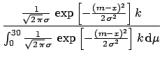
![$\displaystyle \frac{
\frac{1}{\sqrt{2\,\pi}\,\sigma}
\,\exp{\left[-\frac{(m-x)^...
...i}\,\sigma}
\,\exp{\left[-\frac{(m-x)^2}{2\,\sigma^2}\right]}
\,k\, \rm {d}\mu}$](img690.png)
 , and let us limit its domain
to 30, getting
, and let us limit its domain
to 30, getting