- ... length.1.1
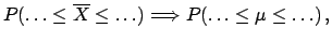
- But after observation
of the first sequence one would strongly suspect that the
coin had two heads, if one had no means of directly checking the coin.
The concept of probability will be used, in fact,
to quantify the degree of such suspicion.
.
.
.
.
.
.
.
.
.
.
.
.
.
.
.
.
.
.
.
.
.
.
.
.
.
.
.
.
.
.
- ... measurand.1.2
- It is then clear
that the definition of true value implying an indefinite series of
measurements with ideal instrumentation gives the illusion that the true
value is unique. The ISO definition, instead, takes into account the fact
that measurements are performed under
real conditions and can be accompanied by all the sources of uncertainty
in the above list.
.
.
.
.
.
.
.
.
.
.
.
.
.
.
.
.
.
.
.
.
.
.
.
.
.
.
.
.
.
.
- ... systematic errors1.3
- To be more precise one should
specify `of unknown size', since an accurately assessed systematic
error does not yield uncertainty, but only a correction to
the raw result.
.
.
.
.
.
.
.
.
.
.
.
.
.
.
.
.
.
.
.
.
.
.
.
.
.
.
.
.
.
.
- ... all''.1.4
- By the way, it is a good and
recommended practice to provide the complete list of
contributions to the overall uncertainty[3];
but it is also clear
that, at some stage, the producer or the user of the result
has to combine the uncertainty to form his idea about the
interval in which the quantity of interest is believed to lie.
.
.
.
.
.
.
.
.
.
.
.
.
.
.
.
.
.
.
.
.
.
.
.
.
.
.
.
.
.
.
- ... require.1.5
- And in fact,
one can see that when there are only two or three
contributions to the `systematic error',
there are still people who
prefer to add them linearly.
.
.
.
.
.
.
.
.
.
.
.
.
.
.
.
.
.
.
.
.
.
.
.
.
.
.
.
.
.
.
- ... justification.1.6
- Some others, including
some old lecture notes of mine, try to convince the reader that the
propagation is applied to the observables, in a very complicated
and artificial way. Then, later, as in the `game of the three cards'
proposed by professional cheaters in the street, one uses the same formulae
for physics quantities, hoping that the students do not notice the
logical gap.
.
.
.
.
.
.
.
.
.
.
.
.
.
.
.
.
.
.
.
.
.
.
.
.
.
.
.
.
.
.
- ... were1.7
- There are also those who express the
result, making the trivial mistake of saying
``this means that, if I repeat the experiment a great
number of times, then I will find that in roughly
68% of the cases the observed
average will be in the interval
![$ \left[\overline{x} - \sigma/\sqrt{n},\
\overline{x} + \sigma/\sqrt{n}\right]''$](img25.png) . (Besides the interpretation
problem, there is a missing factor of
. (Besides the interpretation
problem, there is a missing factor of  in the width of the interval ...)
.
.
.
.
.
.
.
.
.
.
.
.
.
.
.
.
.
.
.
.
.
.
.
.
.
.
.
.
.
.
- ...
that1.8
- The capital letter to indicate the average appearing
in (
![[*]](file:/usr/lib/latex2html/icons/crossref.png) ) is used because here this symbol stands
for a random variable, while in () it indicated a
realization of it. For the Greek symbols this distinction is not made,
but the different role
should be evident from the context.
) is used because here this symbol stands
for a random variable, while in () it indicated a
realization of it. For the Greek symbols this distinction is not made,
but the different role
should be evident from the context.
.
.
.
.
.
.
.
.
.
.
.
.
.
.
.
.
.
.
.
.
.
.
.
.
.
.
.
.
.
.
- ...
value''1.9
- It is worth noting the paradoxical
inversion of role between
 , about which we are in a state of
uncertainty, considered to be a constant, and
the observation
, about which we are in a state of
uncertainty, considered to be a constant, and
the observation
 , which has a certain value
and which is instead considered a random quantity.
This distorted way of thinking
produces the statements to which we are used, such as speaking of ``uncertainty (or error)
on the observed number'': If one observes 10 on a scaler, there is
no uncertainty on this number, but
on the quantity which we try to infer from the observation
(e.g.
, which has a certain value
and which is instead considered a random quantity.
This distorted way of thinking
produces the statements to which we are used, such as speaking of ``uncertainty (or error)
on the observed number'': If one observes 10 on a scaler, there is
no uncertainty on this number, but
on the quantity which we try to infer from the observation
(e.g.  of a Poisson distribution, or a rate).
.
.
.
.
.
.
.
.
.
.
.
.
.
.
.
.
.
.
.
.
.
.
.
.
.
.
.
.
.
.
- ...fig:htest).
1.10
- At present,`
 -values' (or `significance probabilities')
are also ``used in place of hypothesis tests
as a means of giving more information about the relationship between
the data and the hypothesis than does a simple reject/do not
reject decision''[9]. They consist in giving the
probability of the `tail(s)', as also
usually done in HEP, although the
name `-values' has not yet entered our lexicon.
Anyhow, they produce the same interpretation problems of the
hypothesis test paradigm (see also example 8 of next section).
-values' (or `significance probabilities')
are also ``used in place of hypothesis tests
as a means of giving more information about the relationship between
the data and the hypothesis than does a simple reject/do not
reject decision''[9]. They consist in giving the
probability of the `tail(s)', as also
usually done in HEP, although the
name `-values' has not yet entered our lexicon.
Anyhow, they produce the same interpretation problems of the
hypothesis test paradigm (see also example 8 of next section).
.
.
.
.
.
.
.
.
.
.
.
.
.
.
.
.
.
.
.
.
.
.
.
.
.
.
.
.
.
.
- ... prevision1.11
- By prevision I mean, following [11],
a probabilistic `prediction', which corresponds to what is
usually known as expectation value (see Section ).
.
.
.
.
.
.
.
.
.
.
.
.
.
.
.
.
.
.
.
.
.
.
.
.
.
.
.
.
.
.
- ... question,1.12
- Personally,
I find it is somehow impolite to give
an answer to a question which is different
from that asked. At least one should apologize for being
unable to answer the original question. However, textbooks
usually do not do this, and people get confused.
.
.
.
.
.
.
.
.
.
.
.
.
.
.
.
.
.
.
.
.
.
.
.
.
.
.
.
.
.
.
- ... journal.1.13
- Example taken from Ref.
[12].
.
.
.
.
.
.
.
.
.
.
.
.
.
.
.
.
.
.
.
.
.
.
.
.
.
.
.
.
.
.
- ...
true.1.14
- This should not be confused with the probability
of the actual data, which is clearly 1, since they
have been observed.
.
.
.
.
.
.
.
.
.
.
.
.
.
.
.
.
.
.
.
.
.
.
.
.
.
.
.
.
.
.
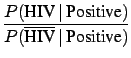
- ... healthy!1.15
- The
result will be a simple application of Bayes' theorem, which will be
introduced later.
A crude way to check this result is to imagine performing the
test on the entire population. Then the number of persons declared
Positive will be all the HIV infected plus
 of the remaining
population. In total 100
of the remaining
population. In total 100  000 infected and 120 000
healthy persons. The general, Bayesian solution is given in
Section
000 infected and 120 000
healthy persons. The general, Bayesian solution is given in
Section
.
.
.
.
.
.
.
.
.
.
.
.
.
.
.
.
.
.
.
.
.
.
.
.
.
.
.
.
.
.
- ...
was:1.16
- One might think that the misleading meaning of
that sentence was due to
unfortunate wording, but this possibility is ruled out by
other statements which show
clearly a quite odd point of view of probabilistic matter.
In fact the DESY 1998 activity report [14] insists
that ``the likelihood that the data produced are the result
of a statistical fluctuation ...is equivalent to that
of tossing a coin and throwing seven heads or tails
in a row'' (replacing `probability' by `likelihood' does
not change the sense of the message).
Then, trying to explain the meaning of a
statistical fluctuation, the following example is given:
``This process can be simulated with a die.
If the number of times a die is
thrown is sufficiently large, the die falls equally often on all faces,
i.e. all six numbers occur equally often. The probability for
each face is exactly a sixth or 16.66%, assuming the die
is not loaded. If the die is thrown less often, then the probability
curve for the distribution of the six die values is no longer a straight
line but has peaks and troughs. The probability distribution
obtained by throwing the die varies about the theoretical value
of 16.66% depending on how many times it is thrown.''
.
.
.
.
.
.
.
.
.
.
.
.
.
.
.
.
.
.
.
.
.
.
.
.
.
.
.
.
.
.
- ... corner.1.17
- One of the odd claims
related to these events was on a poster of an INFN exhibition
at Palazzo delle Esposizioni in Rome: ``These events
are absolutely impossible within the current theory ...
If they will be confirmed, it will imply that....''
Some friends of mine who visited the exhibition
asked me what it meant that ``something impossible
needs to be confirmed''.
.
.
.
.
.
.
.
.
.
.
.
.
.
.
.
.
.
.
.
.
.
.
.
.
.
.
.
.
.
.
- ...
observed?''1.18
- This is as if the conclusion from the AIDS test
depended not only on
 and on the prior probability of being infected,
but also on the probability that this poor
guy experienced events rarer than a mistaken analysis, like
sitting next to Claudia Schiffer
on an international flight,
or winning the lottery, or being hit by a meteorite.
and on the prior probability of being infected,
but also on the probability that this poor
guy experienced events rarer than a mistaken analysis, like
sitting next to Claudia Schiffer
on an international flight,
or winning the lottery, or being hit by a meteorite.
.
.
.
.
.
.
.
.
.
.
.
.
.
.
.
.
.
.
.
.
.
.
.
.
.
.
.
.
.
.
- ...
objection.1.19
- I must admit I have fully understood this point
only very recently, and I thank F. James for having asked,
at the end of the CERN lectures, if I agreed
with the sentence ``The probability of data not observed
is irrelevant in making inferences from an experiment.''[10]
I was not really ready to give a convincing reply, apart from
a few intuitions, and from the trivial comment that this does not mean that
we are not allowed to use MC data
(strictly speaking, frequentists should not use MC data,
as discussed in Section ).
In fact, in the lectures I did not talk about `data+tails', but only
about `data'. This topic will be discussed again in
Section .
.
.
.
.
.
.
.
.
.
.
.
.
.
.
.
.
.
.
.
.
.
.
.
.
.
.
.
.
.
.
- ...
notes.1.20
- As an exercise, to compare the intuitive result with what
we will learn later, it may be interesting to try to calculate,
in the second case of the previous example
(
 ), the value
  such that we would be in a condition
of indifference (i.e. probability 50% each) with respect
to the two generators.
such that we would be in a condition
of indifference (i.e. probability 50% each) with respect
to the two generators.
.
.
.
.
.
.
.
.
.
.
.
.
.
.
.
.
.
.
.
.
.
.
.
.
.
.
.
.
.
.
- ... centuries.2.1
- For example,
it is interesting to report
Einstein's opinion [17] about Hume's criticism:
``Hume saw clearly that certain
concepts, as for example that of causality, cannot be deduced from the
material of experience by logical methods. Kant, thoroughly convinced of
the indispensability of certain concepts, took them - just
as they are selected - to be necessary premises of every kind of
thinking and differentiated them from concepts of empirical origin.
I am convinced, however, that this differentiation is erroneous.''
In the same Autobiographical Notes [17] Einstein,
explaining how he came to the idea of the arbitrary character
of absolute time, acknowledges that
``The type of critical reasoning which was required for the
discovery of this central point was decisively furthered, in my case,
especially by the reading of David Hume's and Ernst Mach's
philosophical writings.'' This tribute to Mach and Hume is
repeated in the `gemeinverständlich' of special relativity
[18]: ``Why is it necessary to drag down from
the Olympian fields of Plato the fundamental ideas
of thought in natural science,
and to attempt to reveal their earthly lineage? Answer: In order
to free these ideas from the taboo attached to them, and thus
to achieve greater freedom in the formation of ideas or concepts.
It is to the immortal credit of D. Hume and E. Mach
that they, above all others, introduced this critical
conception.'' I would like to end this parenthesis
dedicated to Hume with a last citation, this time by
de Finetti[11], closer to the argument of this chapter:
``In the philosophical arena, the problem of
induction, its meaning, use and justification,
has given rise to endless controversy, which, in the absence
of an appropriate probabilistic framework, has inevitably been
fruitless, leaving the major issues unresolved. It seems to me
that the question was correctly formulated by Hume ...
and the pragmatists ... However, the forces of reaction
are always poised, armed with
religious zeal, to defend holy obtuseness against the possibility
of intelligent clarification. No sooner had Hume begun to prise
apart the traditional edifice, then came poor Kant in a desperate attempt
to paper over the cracks and contain the inductive argument
-- like its deductive counterpart -- firmly within the narrow confines
of the logic of certainty.''
.
.
.
.
.
.
.
.
.
.
.
.
.
.
.
.
.
.
.
.
.
.
.
.
.
.
.
.
.
.
- ...
probability.2.2
- Perhaps one may try
to use instead fuzzy logic or something similar. I will
only try to show that this way is productive and leads
to a consistent theory of uncertainty which does not need
continuous injections of extraneous matter. I am
not interested in demonstrating the uniqueness of this
solution, and all
contributions on the subject are welcome.
.
.
.
.
.
.
.
.
.
.
.
.
.
.
.
.
.
.
.
.
.
.
.
.
.
.
.
.
.
.
- ... probability,2.3
- For an introductory
and concise presentation of the subject see also Ref. [21].
.
.
.
.
.
.
.
.
.
.
.
.
.
.
.
.
.
.
.
.
.
.
.
.
.
.
.
.
.
.
- ...
taught2.4
- This remark -- not completely a joke --
is due to the observation that most physicists
interviewed are convinced that () is
legitimate, although they maintain that probability is
the limit of the frequency.
.
.
.
.
.
.
.
.
.
.
.
.
.
.
.
.
.
.
.
.
.
.
.
.
.
.
.
.
.
.
- ...
mechanics2.5
- Without entering into the
open problems of quantum mechanics, let us just say
that it does not matter,
from the cognitive point of view,
whether one believes
that the fundamental laws are intrinsically
probabilistic, or whether this is just due to a limitation of our knowledge,
as hidden variables à la Einstein would imply. If we calculate that
process
 has a probability of 0.9, and process
  0.4, we will
believe much more than .
0.4, we will
believe much more than .
.
.
.
.
.
.
.
.
.
.
.
.
.
.
.
.
.
.
.
.
.
.
.
.
.
.
.
.
.
.
- ... circularity2.6
- Concerning the combinatorial definition,
Poincaré's criticism [6] is remarkable:
``The definition, it will be said, is very simple. The probability of
an event is the ratio of the number of cases favourable to the event
to the total number of possible cases. A simple example will show how
incomplete this definition is: ...
...We are therefore bound to complete the definition by saying
`... to the total number of possible cases, provided the cases are
equally probable.' So we are compelled to define the probable by
the probable. How can we know that two possible cases are equally probable?
Will it be by convention? If we insert at the beginning of every problem
an explicit convention, well and good! We then have nothing to do but to apply
the rules of arithmetic and algebra, and we complete our calculation,
when our result cannot be called in question. But if
we wish to make the slightest application of this result,
we must prove that our convention is legitimate, and we shall find
ourselves in the presence of the very difficulty we thought
we had avoided.''
.
.
.
.
.
.
.
.
.
.
.
.
.
.
.
.
.
.
.
.
.
.
.
.
.
.
.
.
.
.
- ...
arbitrary2.7
- Perhaps this is the reason why
Poincaré [6],
despite his many
brilliant intuitions, above all about the
necessity of the priors (``there are certain points
which seem to be well established. To undertake the calculation of any
probability, and even for that calculation to have any
meaning at all, we must admit, as a point of departure, an
hypothesis or convention which has always
something arbitrary on it ...),
concludes to ``... have set several
problems, and have given no solution ...''. The
coherence makes the distinction between
arbitrariness and `subjectivity' and gives
a real sense to subjective probability.
.
.
.
.
.
.
.
.
.
.
.
.
.
.
.
.
.
.
.
.
.
.
.
.
.
.
.
.
.
.
- ...
recognized2.8
- One should feel obliged to follow
this recommendation as a metrology rule. It is however
remarkable to hear that, in spite of the diffused cultural
prejudices against subjective probability, the scientists of the ISO
working groups have arrived at such a conclusion.
.
.
.
.
.
.
.
.
.
.
.
.
.
.
.
.
.
.
.
.
.
.
.
.
.
.
.
.
.
.
- ... less.2.9
- To understand
the role of implicit prior knowledge, imagine someone
having no scientific or technical education at all, entering
a physics laboratory and reading a number on an
instrument. His scientific knowledge will not improve at all, apart
from the triviality that a given instrument
displayed a number (not much knowledge).
.
.
.
.
.
.
.
.
.
.
.
.
.
.
.
.
.
.
.
.
.
.
.
.
.
.
.
.
.
.
- ... null.2.10
- But also in this case
we have learned something: the thermometer does not work.
.
.
.
.
.
.
.
.
.
.
.
.
.
.
.
.
.
.
.
.
.
.
.
.
.
.
.
.
.
.
- ... `deduction'.2.11
- To be correct, the deduction we
are talking about is different from the classical one. We are dealing,
in fact, with probabilistic deduction, in the sense that,
given a certain cause,
the effect is not univocally determined.
.
.
.
.
.
.
.
.
.
.
.
.
.
.
.
.
.
.
.
.
.
.
.
.
.
.
.
.
.
.
- ... observed.2.12
- It is important to understand that
 can be evaluated before one knows the observed value .
In fact, to be correct,
should be interpreted as
beliefs of under the hypothesis that is observed,
and not only as beliefs of after is observed.
Similarly,
can be evaluated before one knows the observed value .
In fact, to be correct,
should be interpreted as
beliefs of under the hypothesis that is observed,
and not only as beliefs of after is observed.
Similarly,
 can also be built after
the data have been observed, although for teaching purposes the opposite
has been suggested, which corresponds to the most
common case.
can also be built after
the data have been observed, although for teaching purposes the opposite
has been suggested, which corresponds to the most
common case.
.
.
.
.
.
.
.
.
.
.
.
.
.
.
.
.
.
.
.
.
.
.
.
.
.
.
.
.
.
.
- ... of)2.13
- Although I don't believe it, I
leave open the possibility that there really is someone who
has developed some special reasoning to avoid, deep in his mind,
the category of the probable
when figuring out the uncertainty on
a true value.
.
.
.
.
.
.
.
.
.
.
.
.
.
.
.
.
.
.
.
.
.
.
.
.
.
.
.
.
.
.
- ... normal,2.14
- In case of doubt it is
recommended to plot it.
.
.
.
.
.
.
.
.
.
.
.
.
.
.
.
.
.
.
.
.
.
.
.
.
.
.
.
.
.
.
- ... considered2.15
- For a general and self-contained discussion
concerning the inference of the intensity of Poisson processes
at the limit of the detector sensitivity, see Ref. [25].
.
.
.
.
.
.
.
.
.
.
.
.
.
.
.
.
.
.
.
.
.
.
.
.
.
.
.
.
.
.
- ...
events.2.16
- As we shall see, the use of frequencies is absolutely
legitimate in subjective probability, once the distinction between
probability and frequency is properly made. In this case it works
because of the Bernoulli theorem, which states that for a very large
Monte Carlo sample ``it is very improbable
that the frequency distribution
will differ much from the p.d.f.'' (This is the probabilistic
meaning to be attributed to `tend'.)
.
.
.
.
.
.
.
.
.
.
.
.
.
.
.
.
.
.
.
.
.
.
.
.
.
.
.
.
.
.
- ...
 2.17
2.17
- For example,
in the absence of random error the reading (
 )
of a voltmeter depends on the probed voltage (
)
of a voltmeter depends on the probed voltage ( )
and on the scale offset (
)
and on the scale offset ( ):
):
 . Therefore, the result from the
observation of
. Therefore, the result from the
observation of  gives only a constraint between and :
If we know well (within unavoidable uncertainty),
then we can learn something about . If instead the prior knowledge on
is better than that on we can use the measurement
to calibrate the instrument.
gives only a constraint between and :
If we know well (within unavoidable uncertainty),
then we can learn something about . If instead the prior knowledge on
is better than that on we can use the measurement
to calibrate the instrument.
.
.
.
.
.
.
.
.
.
.
.
.
.
.
.
.
.
.
.
.
.
.
.
.
.
.
.
.
.
.
- ... errors.2.18
- But, in order to give
a well-defined probabilistic meaning to
the result, the variations must be performed according
to
 , and not arbitrary.
.
.
.
.
.
.
.
.
.
.
.
.
.
.
.
.
.
.
.
.
.
.
.
.
.
.
.
.
.
.
- ...
`integrate'2.19
- `Integrate' stands
for a generic term which also includes the
approximate method just described.
.
.
.
.
.
.
.
.
.
.
.
.
.
.
.
.
.
.
.
.
.
.
.
.
.
.
.
.
.
.
- ... notes3.1
- Notes based on
lectures given to graduate students in Rome (May 1995)
and summer students at DESY (September 1995).
The original report is Ref. [27]. In this report, notes (indicated by
`Note added' are used, either for clarification or to refer to those
parts not contained in the original `primer'.
.
.
.
.
.
.
.
.
.
.
.
.
.
.
.
.
.
.
.
.
.
.
.
.
.
.
.
.
.
.
- ... will3.2
- The use of the future tense
does not imply that this definition can only be
applied for future events. ``Will occur'' simply
means that the statement ``will be proven to be true'',
even if it refers to the past. Think for example of
``the probability that it was raining in Rome on the day
of the battle of Waterloo''.
.
.
.
.
.
.
.
.
.
.
.
.
.
.
.
.
.
.
.
.
.
.
.
.
.
.
.
.
.
.
- ... reasonable3.3
- This is not always
true in real life. There are also other
practical problems related to betting which have been
treated in the
literature. Other variations of the
definition have also been proposed, like the one
based on the penalization rule. A discussion of the
problem goes beyond the purpose of these notes.
.
.
.
.
.
.
.
.
.
.
.
.
.
.
.
.
.
.
.
.
.
.
.
.
.
.
.
.
.
.
- ... them3.4
- We will talk
later about the influence of a priori beliefs on the
outcome of an experimental investigation.
.
.
.
.
.
.
.
.
.
.
.
.
.
.
.
.
.
.
.
.
.
.
.
.
.
.
.
.
.
.
- ... here3.5
- Very important:
for the meaning of ``the formula of conditional probability''
see Section
.
.
.
.
.
.
.
.
.
.
.
.
.
.
.
.
.
.
.
.
.
.
.
.
.
.
.
.
.
.
- ... occurred3.6
-
 should not be
confused with
should not be
confused with
 , ``the probability that both
events occur''. For example
can be very small, but
nevertheless
very high. Think of the limit case
``
, ``the probability that both
events occur''. For example
can be very small, but
nevertheless
very high. Think of the limit case
`` given '' is a certain event no matter how small
  is,
even if
is,
even if  (in the sense of Section ).
.
.
.
.
.
.
.
.
.
.
.
.
.
.
.
.
.
.
.
.
.
.
.
.
.
.
.
.
.
.
- ...after''3.7
- Note that ``before''
and ``after'' do not really necessarily imply time
ordering, but only the consideration or not of the
new piece of information
.
.
.
.
.
.
.
.
.
.
.
.
.
.
.
.
.
.
.
.
.
.
.
.
.
.
.
.
.
.
- ... probability3.8
- The symbol
 could be misunderstood if one forgets that the proportionality
factor depends on all likelihoods and priors [see ()].
This means that, for a given hypothesis
could be misunderstood if one forgets that the proportionality
factor depends on all likelihoods and priors [see ()].
This means that, for a given hypothesis  ,
as the state of information
,
as the state of information  changes,
 may change
if
may change
if
 and
and
 remain constant, and
if some of the other likelihoods get modified by the new information.
remain constant, and
if some of the other likelihoods get modified by the new information.
.
.
.
.
.
.
.
.
.
.
.
.
.
.
.
.
.
.
.
.
.
.
.
.
.
.
.
.
.
.
- ... ``establishment''3.9
- A case,
concerning
the search for electron compositeness in e
 e
e collisions,
is discussed in Ref. [38].
collisions,
is discussed in Ref. [38].
.
.
.
.
.
.
.
.
.
.
.
.
.
.
.
.
.
.
.
.
.
.
.
.
.
.
.
.
.
.
- ... moment3.10
- For a recent delightful report,
see Ref. [39].
.
.
.
.
.
.
.
.
.
.
.
.
.
.
.
.
.
.
.
.
.
.
.
.
.
.
.
.
.
.
- ... results3.11
- ``A theory
needs to be confirmed by experiments. But it is
also true that an experimental result needs to be confirmed
by a theory.'' This sentence
expresses clearly -- though paradoxically --
the idea that it is difficult to accept a result which is
not rationally justified. An example of results ``not confirmed by
the theory'' are the
 measurements in deep-inelastic scattering
shown in Fig. . Given the conflict
in this situation,
physicists tend to believe more in QCD and use the
``low-'' extrapolations (of what?)
to correct the data for the
unknown values of .
measurements in deep-inelastic scattering
shown in Fig. . Given the conflict
in this situation,
physicists tend to believe more in QCD and use the
``low-'' extrapolations (of what?)
to correct the data for the
unknown values of .
.
.
.
.
.
.
.
.
.
.
.
.
.
.
.
.
.
.
.
.
.
.
.
.
.
.
.
.
.
.
- ... objectivity3.12
- It may look paradoxical,
but, due to the normative role of the coherent bet, the subjective
assessments are more objective about using, without direct responsibility,
someone else is formulae. For example, even the knowledge that
somebody else has a different evaluation of the probability is
new information which must be taken into account.
.
.
.
.
.
.
.
.
.
.
.
.
.
.
.
.
.
.
.
.
.
.
.
.
.
.
.
.
.
.
- ... Laplace3.13
- It may help in understanding
Laplace's approach
if we consider that he called the theory of probability ``good sense
turned into calculation''.
.
.
.
.
.
.
.
.
.
.
.
.
.
.
.
.
.
.
.
.
.
.
.
.
.
.
.
.
.
.
- ... distribution:]4.1
-
The symbols of the following distributions
have the parameters within parentheses to indicate that
the variables are continuous.
.
.
.
.
.
.
.
.
.
.
.
.
.
.
.
.
.
.
.
.
.
.
.
.
.
.
.
.
.
.
- ...
deviation4.2
- Mathematicians and statisticians prefer to
take
 , instead of
  , as
second parameter of the normal distribution. Here the standard deviation
is preferred, since it is homogeneous to and it has
a more immediate physical interpretation. So, one has to pay
attention to be sure about the meaning of expressions
like
, as
second parameter of the normal distribution. Here the standard deviation
is preferred, since it is homogeneous to and it has
a more immediate physical interpretation. So, one has to pay
attention to be sure about the meaning of expressions
like
 .
.
.
.
.
.
.
.
.
.
.
.
.
.
.
.
.
.
.
.
.
.
.
.
.
.
.
.
.
.
.
.
- ...
methods5.1
- This is conceptually what experimentalists
do when they change all the parameters of the Monte Carlo simulation
in order to estimate the ``systematic error''.
.
.
.
.
.
.
.
.
.
.
.
.
.
.
.
.
.
.
.
.
.
.
.
.
.
.
.
.
.
.
- ... variance5.2
- Note added: for
criticisms about the standard treatment of the small-sample problem see Ref.
[].
.
.
.
.
.
.
.
.
.
.
.
.
.
.
.
.
.
.
.
.
.
.
.
.
.
.
.
.
.
.
- ...
notes5.3
- Note added: as is easy to imagine, the
problem of the ``outliers'' should be treated with
care, and surely avoiding automatic prescriptions.
Some hints can be found in Refs. [43] and [44],
and references therein.
.
.
.
.
.
.
.
.
.
.
.
.
.
.
.
.
.
.
.
.
.
.
.
.
.
.
.
.
.
.
- ... mass5.4
- In reality, often
 rather than m is normally distributed.
In this case the terms of the problem change
and a new solution should be worked out, following the
trace indicated in this example.
rather than m is normally distributed.
In this case the terms of the problem change
and a new solution should be worked out, following the
trace indicated in this example.
.
.
.
.
.
.
.
.
.
.
.
.
.
.
.
.
.
.
.
.
.
.
.
.
.
.
.
.
.
.
- ...
procedure,5.5
- We consider detector
and analysis machinery as a black box,
no matter how complicated it is, and treat the numerical
outcome as a result of a direct measurement[1].
.
.
.
.
.
.
.
.
.
.
.
.
.
.
.
.
.
.
.
.
.
.
.
.
.
.
.
.
.
.
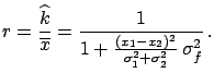
- ... probability''5.6
-
This concept, which is very close to the physicist's mentality,
is not correct from the probabilistic -- cognitive --
point of view. According to the Bayesian scheme, in fact,
the probability changes with the new observations. The final
inference of
 , however, does not depend on the particular sequence
yielding successes over
, however, does not depend on the particular sequence
yielding successes over  trials. This can be seen in the next table
where
trials. This can be seen in the next table
where  is given as a function of the number of trials ,
for the three sequences which give two successes (indicated by ``1'')
in three trials
[the use of () is anticipated]:
is given as a function of the number of trials ,
for the three sequences which give two successes (indicated by ``1'')
in three trials
[the use of () is anticipated]:
| |
Sequence |
| n |
011 |
101 |
110 |
| 0 |
1 |
1 |
1 |
| 1 |
 |
 |
|
| 2 |
 |
|
 |
| 3 |
 |
|
|
This important result, related to the concept of
exchangeability,
``allows'' a physicist who is
reluctant to give up the concept
``unknown constant probability'' to see the problem from his
point of view,
ensuring that the same numerical result is obtained.
.
.
.
.
.
.
.
.
.
.
.
.
.
.
.
.
.
.
.
.
.
.
.
.
.
.
.
.
.
.
- ...
Assuming5.7
- There is a school
of thought according to which the most appropriate
function is
 .
If You think that it is reasonable
for your problem, it may be a good prior.
Claiming that this is ``the Truth'' is one
of the many
claims of the
angels' sex determinations. For didactical purposes
a uniform distribution is more than enough. Some comments
about the
.
If You think that it is reasonable
for your problem, it may be a good prior.
Claiming that this is ``the Truth'' is one
of the many
claims of the
angels' sex determinations. For didactical purposes
a uniform distribution is more than enough. Some comments
about the  prescription will be given
when discussing the particular case
prescription will be given
when discussing the particular case  .
.
Note added: criticisms concerning so called ``reference priors''
can be found in Ref.[].
.
.
.
.
.
.
.
.
.
.
.
.
.
.
.
.
.
.
.
.
.
.
.
.
.
.
.
.
.
.
- ...
Integrating5.8
- It may help to know that
.
.
.
.
.
.
.
.
.
.
.
.
.
.
.
.
.
.
.
.
.
.
.
.
.
.
.
.
.
.
- ... values6.1
- The choice of the adjective
``raw'' will become clearer later on.
.
.
.
.
.
.
.
.
.
.
.
.
.
.
.
.
.
.
.
.
.
.
.
.
.
.
.
.
.
.
- ...
completely6.2
- Note added: for criticisms about
the standard treatment of the small-sample problem see Ref. [].
.
.
.
.
.
.
.
.
.
.
.
.
.
.
.
.
.
.
.
.
.
.
.
.
.
.
.
.
.
.
- ... quantity6.3
-
By ``input quantity'' the ISO Guide means
any of the contributions
 or
or  which enter into () and ().
.
.
.
.
.
.
.
.
.
.
.
.
.
.
.
.
.
.
.
.
.
.
.
.
.
.
.
.
.
.
- ... deviation6.4
- This example shows a type B
uncertainty originated by random errors.
.
.
.
.
.
.
.
.
.
.
.
.
.
.
.
.
.
.
.
.
.
.
.
.
.
.
.
.
.
.
- ... methods6.5
- Note added: This is exactly the
presumed paradox reported by the 1998 issue of the
PDG[46]
as an argument against Bayesian statistics (Section 29.6.2, p. 175:
``If Bayesian estimates are averaged, they do not
converge to the true value,
since they have all been forced to be positive'').
.
.
.
.
.
.
.
.
.
.
.
.
.
.
.
.
.
.
.
.
.
.
.
.
.
.
.
.
.
.
- ... variables6.6
-
To make the formalism lighter, let us call
both the
random variable associated with the quantity and the quantity itself
by the same name
 (instead of
  ).
).
.
.
.
.
.
.
.
.
.
.
.
.
.
.
.
.
.
.
.
.
.
.
.
.
.
.
.
.
.
.
- ... quantities6.7
-
In this section[47]
the symbol will indicate
the variable associated to the
 -th physical quantity
and
-th physical quantity
and  its
its  -th direct measurement;
  the best estimate of
its value, obtained by an average over many direct measurements or
indirect measurements,
the best estimate of
its value, obtained by an average over many direct measurements or
indirect measurements,  the
standard deviation, and
the
standard deviation, and 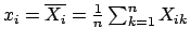 the value corrected for the calibration
constants. The weighted average of several will be
denoted by
.
the value corrected for the calibration
constants. The weighted average of several will be
denoted by
.
.
.
.
.
.
.
.
.
.
.
.
.
.
.
.
.
.
.
.
.
.
.
.
.
.
.
.
.
.
.
- ...
covariance6.8
- Note added: The
``
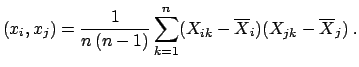 '' at the denominator of ()
is for the same reason as the ``'' of the sample standard deviation.
Although I do not agree with the rationale behind it, this formula can
be considered a kind of standard and, anyhow, replacing ``'' by ``''
has no effect in normal applications. As already said, in these notes
I will not discuss the small-sample problem; anyone is interested in my
worries concerning default formulae for small samples, as
well as Student t distribution may have a look at Ref. [].
'' at the denominator of ()
is for the same reason as the ``'' of the sample standard deviation.
Although I do not agree with the rationale behind it, this formula can
be considered a kind of standard and, anyhow, replacing ``'' by ``''
has no effect in normal applications. As already said, in these notes
I will not discuss the small-sample problem; anyone is interested in my
worries concerning default formulae for small samples, as
well as Student t distribution may have a look at Ref. [].
.
.
.
.
.
.
.
.
.
.
.
.
.
.
.
.
.
.
.
.
.
.
.
.
.
.
.
.
.
.
- ... harmless6.9
-
This can be seen by
rewriting () as
For any
 ,
the first two terms determine the value of , and the
third one binds to 1.
,
the first two terms determine the value of , and the
third one binds to 1.
.
.
.
.
.
.
.
.
.
.
.
.
.
.
.
.
.
.
.
.
.
.
.
.
.
.
.
.
.
.
- ... effects7.1
- The
broadening of the distribution due to the smearing suggests
a choice of
 larger than
  . It is worth mentioning
that there is no need to reject events where a measured quantity
has a value outside the range allowed for the physical quantity.
For example, in the case of
deep-inelastic scattering events, cells with
. It is worth mentioning
that there is no need to reject events where a measured quantity
has a value outside the range allowed for the physical quantity.
For example, in the case of
deep-inelastic scattering events, cells with
 or
or
 give information
about the true distribution too.
give information
about the true distribution too.
.
.
.
.
.
.
.
.
.
.
.
.
.
.
.
.
.
.
.
.
.
.
.
.
.
.
.
.
.
.
- ... inefficiency7.2
- If
 then
then
 will
be set to zero, since the experiment is not sensitive to the cause
will
be set to zero, since the experiment is not sensitive to the cause  .
.
.
.
.
.
.
.
.
.
.
.
.
.
.
.
.
.
.
.
.
.
.
.
.
.
.
.
.
.
.
.
- ...
events8.1
- Please note that `event' is also
used here according to HEP jargon (this is quite a case of
homonymy to which one has to pay attention, but it has
nothing to do with the linguistic schizophrenia I am talking about).
.
.
.
.
.
.
.
.
.
.
.
.
.
.
.
.
.
.
.
.
.
.
.
.
.
.
.
.
.
.
- ...
belief.8.2
- In fact, one could use the combinatorial evaluation
in point 6 as well, because of the discussed cultural reasons,
but not everybody
is willing to speak about the probability of something
which has a very precise
value, although unknown.
.
.
.
.
.
.
.
.
.
.
.
.
.
.
.
.
.
.
.
.
.
.
.
.
.
.
.
.
.
.
- ... confusion.8.3
- See for example Refs. [46] and
[60], where it is admitted that the Bayesian approach is good for decision problems, although they
stick to the frequentistic approach.
.
.
.
.
.
.
.
.
.
.
.
.
.
.
.
.
.
.
.
.
.
.
.
.
.
.
.
.
.
.
- ... bet8.4
- This corresponds to a
probability of
 .
.
.
.
.
.
.
.
.
.
.
.
.
.
.
.
.
.
.
.
.
.
.
.
.
.
.
.
.
.
.
.
- ... bag.8.5
- Sometimes this expectation is justified
advocating the law of large numbers, expressed by the
Bernoulli theorem. This is unacceptable, as pointed out by
de Finetti: ``For those who seek to connect the notion of probability
with that of frequency,
results which relate probability and frequency
in some way (and especially those
results like the `law of large numbers') play a pivotal rôle,
providing support for the approach and for the identification
of the concepts. Logically speaking, however, one cannot escape
from the dilemma posed by the fact that the same thing cannot both
be assumed first as a definition and then proved as a theorem; nor
can one avoid the contradiction that arises from a definition which
would assume as certain something that the theorem only states
to be very probable.''[11]
.
.
.
.
.
.
.
.
.
.
.
.
.
.
.
.
.
.
.
.
.
.
.
.
.
.
.
.
.
.
- ... objectivity.8.6
- My preferred motto on this matter
is ``no one should be allowed to speak about
objectivity unless he has had 10-20 years working
experience in frontier science, economics, or any other applied field''.
.
.
.
.
.
.
.
.
.
.
.
.
.
.
.
.
.
.
.
.
.
.
.
.
.
.
.
.
.
.
- ...
too.8.7
- For example, the statistician
D. Berry[63]
has amused himself by counting how many times Hawking uses
`belief', `to believe', or synonyms, in his `A brief
history of time'. The book could have been entitled `A brief
history of beliefs', pointed out Berry in his talk...
.
.
.
.
.
.
.
.
.
.
.
.
.
.
.
.
.
.
.
.
.
.
.
.
.
.
.
.
.
.
- ... information.8.8
- Recently, I met
an elderly physicist at the meeting of the Italian Physical Society,
who was nostalgic about the good old times when we could see
 decay in emulsions,
and complained that at present the sophisticated electronic experiments
are based on models. It took me a while to convince
him that in emulsions as well
he had a model and that he was not seeing these particles either.
decay in emulsions,
and complained that at present the sophisticated electronic experiments
are based on models. It took me a while to convince
him that in emulsions as well
he had a model and that he was not seeing these particles either.
.
.
.
.
.
.
.
.
.
.
.
.
.
.
.
.
.
.
.
.
.
.
.
.
.
.
.
.
.
.
- ...
physicists8.9
- Outstanding physicists have no reluctance
in talking explicitly about beliefs. Then, paradoxically,
objective science is for those who avoid the word `belief'
nothing but the set of beliefs of the influential scientists
to which they believe...
.
.
.
.
.
.
.
.
.
.
.
.
.
.
.
.
.
.
.
.
.
.
.
.
.
.
.
.
.
.
- ... estimators8.10
- It is worth
remembering that, in the Bayesian approach, the complete answer is given by
the final distribution. The prevision (`expected value')
is just a way
of summarizing the result, together with the standard uncertainty.
Besides motivations based on penalty rules, which we cannot
discuss, a practical justification is that what matters for any further
approximated analysis, are expected values and
standard deviation, whose properties are used in
uncertainty propagation. There is nothing wrong in providing
the mode(s) of the distribution or any other quantity one finds it
sensible to summarize
 as well.
.
.
.
.
.
.
.
.
.
.
.
.
.
.
.
.
.
.
.
.
.
.
.
.
.
.
.
.
.
.
- ... use8.11
- I refer to the steps followed in the proof
of Bayes' theorem given in
Section . They should
convince the reader that
 calculated
in this way is the best we can say about
calculated
in this way is the best we can say about  .
Some say that in the Bayesian inference the answer is the answer
(I have heard this sentence from A. Smith at the Valencia-6 conference),
in the sense that one can use all his best knowledge
to evaluate the probability of an event, but then, whatever happens,
cannot change the assessed probability, but, at most, it can -- and must --
be taken into account for the next assessment of a
different,
although analogous event.
.
.
.
.
.
.
.
.
.
.
.
.
.
.
.
.
.
.
.
.
.
.
.
.
.
.
.
.
.
.
- ... work!8.12
- This is an actual statement I have heard by
Monte Carlo-oriented HEP yuppies.
.
.
.
.
.
.
.
.
.
.
.
.
.
.
.
.
.
.
.
.
.
.
.
.
.
.
.
.
.
.
- ...
nonsense,8.13
- Zech says, more optimistically: ``Coverage is the
magic objective of classical confidence bounds. It is an attractive
property from a purely esthetic point of view but it is not obvious
how to make use of this concept.''[67]
.
.
.
.
.
.
.
.
.
.
.
.
.
.
.
.
.
.
.
.
.
.
.
.
.
.
.
.
.
.
- ... quotation8.14
- The translation of the symbols
is as follows:
 stands for the measured quantity
( or
stands for the measured quantity
( or
 in these notes);
 stands for the true value ( or here);
 for
for
 .
.
.
.
.
.
.
.
.
.
.
.
.
.
.
.
.
.
.
.
.
.
.
.
.
.
.
.
.
.
.
.
- ...
imply.8.15
- One would object that this is, more or less,
the result that we could obtain making a Bayesian analysis
with a uniform prior. But it was said that this prior
assumes a positive attitude of the experimenters,
i.e. that the experiment was planned, financed, and operated
by rational people, with the hope of observing something
(see Sections and ).
This topic, together with the issue of reporting experimental results
in a prior-free way, is discussed in detail in Ref. [25].
.
.
.
.
.
.
.
.
.
.
.
.
.
.
.
.
.
.
.
.
.
.
.
.
.
.
.
.
.
.
- ...
distribution8.16
- The necessity of using integrated distributions
is due to the fact that
the probability of observing a particular configuration is
always very small,
and a frequentistic test would reject the
null hypotheses.
.
.
.
.
.
.
.
.
.
.
.
.
.
.
.
.
.
.
.
.
.
.
.
.
.
.
.
.
.
.
- ...
before.8.17
- See Section .
.
.
.
.
.
.
.
.
.
.
.
.
.
.
.
.
.
.
.
.
.
.
.
.
.
.
.
.
.
.
- ...
abstract8.18
- I quote here the original abstract, which appears
on page 18
of the conference abstract book.
.
.
.
.
.
.
.
.
.
.
.
.
.
.
.
.
.
.
.
.
.
.
.
.
.
.
.
.
.
.
- ... experiment?''.8.19
- I also made
other comments on the general illogicality of his arguments,
which you may easily imagine by reading the abstract. For these
comments I even received applause from the audience, which
really surprised me, until I learned that David Moore is one of the
most authoritative American statisticians: only a outsider like me
would have said what I said...
.
.
.
.
.
.
.
.
.
.
.
.
.
.
.
.
.
.
.
.
.
.
.
.
.
.
.
.
.
.
- ...
verifiability.8.20
- It is
interesting to realize, in the light of this reflection, that
the ISO definition of true value (``a value compatible with the
definition of a given particular quantity'', see
Sections and
)
can accommodate this point of view.
.
.
.
.
.
.
.
.
.
.
.
.
.
.
.
.
.
.
.
.
.
.
.
.
.
.
.
.
.
.
- ...
normalized.8.21
- I have made use several times
in these notes of improper distributions, i.e. such that

d
but, as specified, they were always thought to be the limit of
proper distributions (see, for example, Section ).
.
.
.
.
.
.
.
.
.
.
.
.
.
.
.
.
.
.
.
.
.
.
.
.
.
.
.
.
.
.
- ...
similar8.22
- There is nothing profound in the fact that the
two cases give very similar results. It is just due to the numbers
of these examples (i.e.
 ).
).
.
.
.
.
.
.
.
.
.
.
.
.
.
.
.
.
.
.
.
.
.
.
.
.
.
.
.
.
.
.
- ...
reasonable9.1
- I insist on the
fact that they must be reasonable,
and not just any prior.
The fact that absurd priors give absurd results
does not invalidate the inferential framework based on
subjective probability.
.
.
.
.
.
.
.
.
.
.
.
.
.
.
.
.
.
.
.
.
.
.
.
.
.
.
.
.
.
.
- ... translated9.2
- This two-step
inference is not really needed, but it helps to follow the
inferential flow. One could think more directly of
When the dependence between the two quantities is not
linear, a two-step inference may cause trouble: see comments
in Section .
.
.
.
.
.
.
.
.
.
.
.
.
.
.
.
.
.
.
.
.
.
.
.
.
.
.
.
.
.
.
- ...
code9.3
- If you are interested in Bayesian analysis with
Mathematica you may take a look at Refs.
[81] and [82]
(I take for responsibility on the quality of the products, as I have
never used them).
.
.
.
.
.
.
.
.
.
.
.
.
.
.
.
.
.
.
.
.
.
.
.
.
.
.
.
.
.
.
- ...
game.9.4
- This section is intentionally pedagogical.
An analysis using the best physical assumptions can be found
in Ref. [26]. Indeed, this analysis follows the strategy
outlined here, with some
variations introduced to match the information available in
the real situation.
.
.
.
.
.
.
.
.
.
.
.
.
.
.
.
.
.
.
.
.
.
.
.
.
.
.
.
.
.
.
- ...
inference9.5
- A two-step inference was shown
in Section for the case
of monopole search. There there was no problem
because and
 are linearly related.
.
.
.
.
.
.
.
.
.
.
.
.
.
.
.
.
.
.
.
.
.
.
.
.
.
.
.
.
.
.
- ... LEONES''9.6
- ``Here are the lions''
is what the ancient Romans used to write on the parts of
their maps representing unexplored regions.
.
.
.
.
.
.
.
.
.
.
.
.
.
.
.
.
.
.
.
.
.
.
.
.
.
.
.
.
.
.
- ...
becomes9.7
- Numerologists may complain that this does not correspond
to exactly 95%, but the same happens when a
standard uncertainty is rounded to one or two digits
and the probability level calculated from the rounded number
may differ a lot from the nominal 68.3% calculated
from the original value. But who cares?
.
.
.
.
.
.
.
.
.
.
.
.
.
.
.
.
.
.
.
.
.
.
.
.
.
.
.
.
.
.
![$\displaystyle \int_{-\infty}^{+\infty}\exp{\left[b\,x-\frac{x^2}{a^2}\right]}\,\rm {d}x
= \sqrt{a^2\,\pi}\,\exp{\left[\frac{a^2\,b^2}{4}\right]}\,.$](img831.png)