


Next: Approximate methods
Up: Evaluation of uncertainty: general
Previous: Indirect measurements
Contents
Systematic errors
Uncertainty due to systematic effects
is also included in a natural way in this approach.
Let us first define the notation ( is the generic index):
-
 is the
`n-tuple' (vector) of observables
is the
`n-tuple' (vector) of observables
 ;
;
-
 is the
n-tuple of true values
is the
n-tuple of true values
 ;
;
-
 is the
n-tuple of influence quantities
is the
n-tuple of influence quantities  .
.
By influence quantities we mean:
-

- all kinds of external factors which
may influence the result (temperature, atmospheric
pressure, etc.);
-
- all calibration constants;
-
- all possible hypotheses upon
which the results may depend (e.g.
Monte Carlo parameters).
From a probabilistic point of view, there
is no distinction between
 and
and
 : they are all conditional
hypotheses for the
: they are all conditional
hypotheses for the
 , i.e. causes
which produce the observed effects. The difference
is simply that we are interested in
rather than
in
, i.e. causes
which produce the observed effects. The difference
is simply that we are interested in
rather than
in
 2.17
2.17
There are alternative ways to take
into account
the systematic effects in the final distribution of
:
- Global inference on
 .
We can use Bayes' theorem to make an
inference
on
and
,
as described in Section
.
We can use Bayes' theorem to make an
inference
on
and
,
as described in Section ![[*]](file:/usr/lib/latex2html/icons/crossref.png) :
This method, depending on the joint prior distribution
:
This method, depending on the joint prior distribution
 , can
even model possible correlations between
and
(e.g. radiative correction depending on the
quantity of interest).
, can
even model possible correlations between
and
(e.g. radiative correction depending on the
quantity of interest).
- Conditional inference (see Fig. ).
Figure:
Model to handle the uncertainty due to systematic errors
by the use of conditional probability.
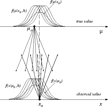 |
Given the observed data, one has a joint distribution
of
for all possible configurations
of
:
Each conditional result is reweighed with the distribution
of beliefs of
, using the well-known law
of probability:
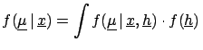 d d |
(2.6) |
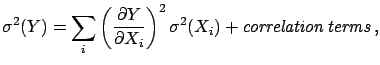
- Propagation of uncertainties. Essentially, one applies
the propagation of uncertainty, whose most general case
has been illustrated in
the previous section, making use of the following model:
One considers a raw result on raw values
 for some nominal values of the influence quantities,
i.e.
then (corrected) true values are obtained as a function
of the raw ones and of the possible values of the influence quantities,
i.e.
for some nominal values of the influence quantities,
i.e.
then (corrected) true values are obtained as a function
of the raw ones and of the possible values of the influence quantities,
i.e.
The three ways lead to the same result and each of them can be more
or less intuitive to different people,
and more less suitable for different applications.
For example, the last two, which are formally equivalent,
are the most intuitive for HEP experimentalists,
and it is conceptually equivalent to what they do
when they vary -- within
reasonable intervals -- all Monte Carlo
parameters in order to estimate the
systematic errors.2.18
The third form is particularly convenient to make linear
expansions which lead to approximated solutions (see
Section ).
There is an important remark to be made.
In some cases it is preferable not to
`integrate'2.19 over
all  's. Instead, it is better to report
the result as
's. Instead, it is better to report
the result as
 ,
where
,
where  stands for a subset
of
, taken at their nominal values,
if:
stands for a subset
of
, taken at their nominal values,
if:
- could be controlled better by the users
of the result (for example
 is a theoretical
quantity on which there is work in progress);
is a theoretical
quantity on which there is work in progress);
- there is some chance of achieving a better knowledge
of within the same experiment (for example
 could be the overall calibration constant
of a calorimeter);
could be the overall calibration constant
of a calorimeter);
- a discrete and small number of very different
hypotheses could affect the result. For example:
This is, in fact, the standard way in which this
kind of result has been presented (apart from the inessential fact
that only best values and standard deviations
are given, assuming normality).
If results are presented under the
condition of , one should also report
the derivatives of
with
respect to the result, so that one does
not have to redo the complete analysis when the influence
factors are better known. A typical example
in which this is usually done is the possible
variation of the result due to the precise values
of the charm-quark mass. A recent example in which this idea has been applied
thoroughly is given in Ref. [26].
Next: Approximate methods
Up: Evaluation of uncertainty: general
Previous: Indirect measurements
Contents
Giulio D'Agostini
2003-05-15