Next: Peelle's Pertinent Puzzle
Up: Use and misuse of
Previous: Offset uncertainty
Contents
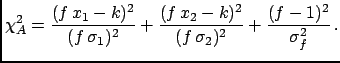
Let
 and
and
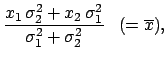
 be the two measured values,
and
be the two measured values,
and  the common standard uncertainty on the scale:
where
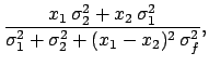 .
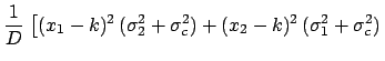
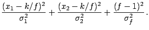
We obtain in this case the following result:
.
We obtain in this case the following result:
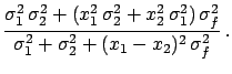
With respect to the previous case,
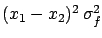 has a new term
 in the denominator. As long as
this is negligible with respect to the individual variances
we still get the weighted average
in the denominator. As long as
this is negligible with respect to the individual variances
we still get the weighted average
 ,
otherwise a smaller value is obtained.
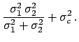
Calling
,
otherwise a smaller value is obtained.
Calling 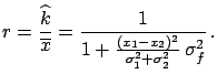 the ratio between
and
, we obtain
the ratio between
and
, we obtain
 |
(6.54) |
Written in this way, one can see that the deviation from the
simple average value depends on the compatibility of the two values
and on the normalization uncertainty.
This can be understood in the following way:
as soon as the two values are in some disagreement, the fit
starts to vary the normalization factor
(in a hidden way)
and to squeeze the scale
by an amount allowed by , in order to minimize the
 .
The reason the fit prefers
normalization factors smaller than 1
under these conditions
lies in the standard formalism of the covariance propagation,
where only first derivatives are considered. This
implies that the individual
standard deviations are not rescaled by lowering the normalization
factor, but
the points get closer.
.
The reason the fit prefers
normalization factors smaller than 1
under these conditions
lies in the standard formalism of the covariance propagation,
where only first derivatives are considered. This
implies that the individual
standard deviations are not rescaled by lowering the normalization
factor, but
the points get closer.
- Example 1.
- Consider
the results of two measurements,
 and
and
 , having
a
, having
a  common normalization error.
Assuming that the two measurements
refer to the same physical quantity,
the best estimate
of its true value can be obtained
by fitting the points to a constant.
Minimizing
with
common normalization error.
Assuming that the two measurements
refer to the same physical quantity,
the best estimate
of its true value can be obtained
by fitting the points to a constant.
Minimizing
with
 estimated empirically by the data, as explained
in the previous section, one obtains a value of
estimated empirically by the data, as explained
in the previous section, one obtains a value of
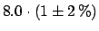
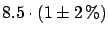
 , which is surprising to say the least,
since the most
probable result is outside the interval determined by the two
measured values.
, which is surprising to say the least,
since the most
probable result is outside the interval determined by the two
measured values.
- Example 2.
- A real life
case of this strange effect which occurred during
the global analysis of the
 ratio in
 performed by The CELLO Collaboration[48],
is shown in
Fig.
performed by The CELLO Collaboration[48],
is shown in
Fig. ![[*]](file:/usr/lib/latex2html/icons/crossref.png) .
The data points represent the averages in
energy bins of the results of the PETRA and PEP experiments. They
are all correlated and
the bars show the
total uncertainty
(see Ref. [48] for details). In particular, at the
intermediate stage of the analysis shown in the figure, an
overall
.
The data points represent the averages in
energy bins of the results of the PETRA and PEP experiments. They
are all correlated and
the bars show the
total uncertainty
(see Ref. [48] for details). In particular, at the
intermediate stage of the analysis shown in the figure, an
overall  systematic error due theoretical uncertainties
was included in the covariance matrix.
The values above
systematic error due theoretical uncertainties
was included in the covariance matrix.
The values above  GeV
show the first hint of the rise of the
cross-section
due to the
GeV
show the first hint of the rise of the
cross-section
due to the  pole.
At that time it was
very interesting to prove that the observation was not
just a statistical fluctuation.
In order to test this, the
measurements were fitted with
a theoretical function having no
contributions,
using only data below a certain energy.
It was expected that a fast increase of
per number of degrees of freedom
pole.
At that time it was
very interesting to prove that the observation was not
just a statistical fluctuation.
In order to test this, the
measurements were fitted with
a theoretical function having no
contributions,
using only data below a certain energy.
It was expected that a fast increase of
per number of degrees of freedom  would be observed
above GeV,
indicating that a theoretical prediction without
would be inadequate for describing the high-energy data.
The surprising result
was a ``repulsion''
(see Fig. )
between the experimental data and the fit:
Including the high-energy points with larger a lower
curve was obtained,
while
would be observed
above GeV,
indicating that a theoretical prediction without
would be inadequate for describing the high-energy data.
The surprising result
was a ``repulsion''
(see Fig. )
between the experimental data and the fit:
Including the high-energy points with larger a lower
curve was obtained,
while
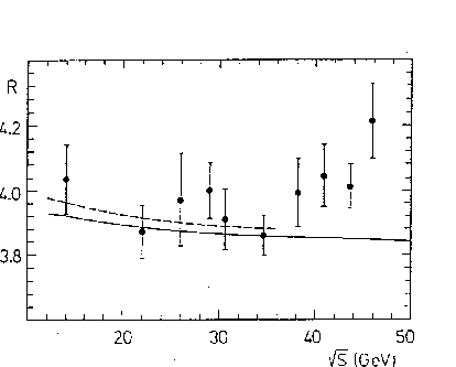 remained almost constant.
Figure:
R measurements
from PETRA and PEP experiments
with the best fits
of QED+QCD to all the data (full line) and only below
GeV (dashed line). All data points are correlated (see text).
 |
To see the source
of this effect more explicitly let us consider an alternative way
often used to take
the normalization uncertainty
into account.
A scale factor  , by which all
data points are multiplied, is introduced to the
expression of the :
, by which all
data points are multiplied, is introduced to the
expression of the :
 |
(6.55) |
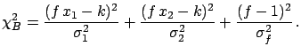
Let us also consider the same expression when the individual
standard deviations
are not rescaled:
 |
(6.56) |
The use of  always gives the result
 ,
because the term
,
because the term
 is harmless6.9 as far as the value of the minimum
and the determination on
are concerned.
Its only influence is
on
is harmless6.9 as far as the value of the minimum
and the determination on
are concerned.
Its only influence is
on
 , which turns out to be equal to
quadratic combination of the
weighted average standard deviation with
, which turns out to be equal to
quadratic combination of the
weighted average standard deviation with
 ,
the normalization uncertainty on the
average.
This result corresponds to the usual one
when the normalization factor
in the definition of is not included,
and the overall uncertainty is added
at the end.
,
the normalization uncertainty on the
average.
This result corresponds to the usual one
when the normalization factor
in the definition of is not included,
and the overall uncertainty is added
at the end.
Instead,
the use of  is equivalent to the
covariance matrix: The same values of the minimum ,
of
and of
are obtained, and
is equivalent to the
covariance matrix: The same values of the minimum ,
of
and of
are obtained, and
 at the minimum turns out to be exactly the ratio
defined above. This demonstrates that the effect happens
when the data values are rescaled independently of their
standard uncertainties. The effect can become huge if the
data show mutual disagreement.
The equality of the results obtained with
with those obtained with the covariance matrix allows us to
study, in a simpler way,
the behaviour of (=
)
when an arbitrary number of data points are analysed.
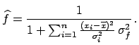
The fitted value of the normalization factor is
at the minimum turns out to be exactly the ratio
defined above. This demonstrates that the effect happens
when the data values are rescaled independently of their
standard uncertainties. The effect can become huge if the
data show mutual disagreement.
The equality of the results obtained with
with those obtained with the covariance matrix allows us to
study, in a simpler way,
the behaviour of (=
)
when an arbitrary number of data points are analysed.
The fitted value of the normalization factor is
 |
(6.57) |
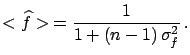
If the values of  are consistent with
a common
true value it can be shown
that the expected value of
is
are consistent with
a common
true value it can be shown
that the expected value of
is
 |
(6.58) |
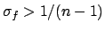
Hence, there is a bias on the result when for a non-vanishing
a large number of data points are fitted. In particular,
the fit on average produces a bias larger than the
normalization uncertainty itself if
 .
One can also see that
.
One can also see that
 and the
minimum of
obtained with the
covariance matrix or with are smaller by the same factor
than those obtained with .
and the
minimum of
obtained with the
covariance matrix or with are smaller by the same factor
than those obtained with .
Next: Peelle's Pertinent Puzzle
Up: Use and misuse of
Previous: Offset uncertainty
Contents
Giulio D'Agostini
2003-05-15