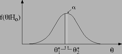
A frequentistic hypothesis test follows the
scheme outlined below (see Fig. ![]() ).
1.10
).
1.10
| (1.6) |
The usual justification for the procedure
is that the probability ![]() is so low that it is
practically impossible for the test variable to fall
outside the interval. Then, if this event
happens, we have good reason to reject the
hypothesis.
is so low that it is
practically impossible for the test variable to fall
outside the interval. Then, if this event
happens, we have good reason to reject the
hypothesis.
One can recognize behind this reasoning a revised version of the classical `proof by contradiction' (see, e.g., Ref. [10]). In standard dialectics, one assumes a hypothesis to be true and looks for a logical consequence which is manifestly false in order to reject the hypothesis. The slight difference is that in the hypothesis test scheme, the false consequence is replaced by an improbable one. The argument may look convincing, but it has no grounds. In order to analyse the problem well, we need to review the logic of uncertainty. For the moment a few examples are enough to indicate that there is something troublesome behind the procedure.
![$ [\theta_1^*,\theta_2^*]$](img60.png) around the expected
value of
around the expected
value of | (1.7) |
One may object that the reason is not only the small probability
of the rejection region, but also its distance from the
expected value. Figure ![]() is an example
against this objection.
is an example
against this objection.
E![$\displaystyle \left[\overline{X}_{300}\right]$](img65.png) |
(1.8) | ||
| (1.9) |
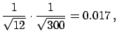 normally distributed
because of the central limit theorem.
This means that there is 99% probability that an average
will come out in the interval
normally distributed
because of the central limit theorem.
This means that there is 99% probability that an average
will come out in the interval
| (1.10) |
``the hypothesisi.e. one receives a precise answer to a different question. In fact, the meaning of the previous statement is simply= `no mistakes' is rejected at the 1% level of significance'',
``there is only a 1% probability that the average falls outside the selected interval, if the calculations were done correctly''.But this does not answer our natural question,1.12 i.e. that concerning the probability of mistake, and not that of results far from the average if there were no mistakes. Moreover, the statement sounds as if one would be 99% sure that the student has made a mistake! This conclusion is highly misleading.
How is it possible, then, to answer the very question concerning the probability of mistakes? If you ask the students (before they take a standard course in hypothesis tests) you will hear the right answer, and it contains a crucial ingredient extraneous to the logic of hypothesis tests:
``It all depends on who has made the calculation!''In fact, if the calculation was done by a well-tested program the probability of mistake would be zero. And students know rather well their probability of making mistakes.
A scientific journal changes its publication policy.
The editors announce that results with a significance level of
5% will no longer be accepted. Only those with a level
of ![]() will be published. The rationale for the change,
explained in an editorial,
looks reasonable and it can be shared without
hesitation: ``We want to publish only good results.''
will be published. The rationale for the change,
explained in an editorial,
looks reasonable and it can be shared without
hesitation: ``We want to publish only good results.''
1000 experimental physicists, not convinced by this severe rule, conspire against the journal. Each of them formulates a wrong physics hypothesis and performs an experiment to test it according to the accepted/rejected scheme.
Roughly 10 physicists get ![]() significant results. Their papers
are accepted and published. It follows that, contrary to
the wishes of the editors, the first issue of the journal under
the new policy contains only wrong results!
significant results. Their papers
are accepted and published. It follows that, contrary to
the wishes of the editors, the first issue of the journal under
the new policy contains only wrong results!
The solution to the kind of paradox raised by this example seems clear: The physicists knew with certainty that the hypotheses were wrong. So the example looks like an odd case with no practical importance. But in real life who knows in advance with certainty if a hypothesis is true or false?