


Next: Misunderstandings caused by the
Up: Uncertainty in physics and
Previous: Probability of the causes
Contents
Unsuitability of confidence intervals
According to the standard theory of probability,
statement (![[*]](file:/usr/lib/latex2html/icons/crossref.png) ) is nonsense, and, in fact,
good frequentistic books do not include it.
They speak instead
about `confidence intervals', which have a completely
different interpretation [that of ()],
although several books and many
teachers suggest
an interpretation of these intervals as if they were
probabilistic statements on the true values, like ().
But it seems to me that
it is practically impossible, even for those who are fully
aware of the frequentistic theory,
to avoid misleading conclusions.
This opinion is well stated by Howson and Urbach in
a paper to Nature[8]:
) is nonsense, and, in fact,
good frequentistic books do not include it.
They speak instead
about `confidence intervals', which have a completely
different interpretation [that of ()],
although several books and many
teachers suggest
an interpretation of these intervals as if they were
probabilistic statements on the true values, like ().
But it seems to me that
it is practically impossible, even for those who are fully
aware of the frequentistic theory,
to avoid misleading conclusions.
This opinion is well stated by Howson and Urbach in
a paper to Nature[8]:
``The statement that such-and-such is a 95% confidence interval
for  seems objective. But what does it say?
It may be imagined that a 95% confidence
interval corresponds to a 0.95 probability
that the unknown parameter lies in the confidence range.
But in the classical approach, is not a
random variable, and so
has no probability. Nevertheless, statisticians
regularly say that one can be `95% confident' that
the parameter lies in the confidence interval.
They never say why.''
seems objective. But what does it say?
It may be imagined that a 95% confidence
interval corresponds to a 0.95 probability
that the unknown parameter lies in the confidence range.
But in the classical approach, is not a
random variable, and so
has no probability. Nevertheless, statisticians
regularly say that one can be `95% confident' that
the parameter lies in the confidence interval.
They never say why.''
The origin of the problem goes directly to the
underlying concept of probability. The frequentistic concept of confidence
interval is, in fact, a kind of artificial invention to
characterize the uncertainty consistently with the
frequency-based definition of probability. But, unfortunately
- as a matter of fact - this attempt to classify the state of
uncertainty (on the true value) trying to avoid the
concept of probability of hypotheses
produces misinterpretation.
People tend to
turn arbitrarily
() into ()
with an intuitive reasoning that
I like to paraphrase as `the dog and the hunter':
We know that a dog has a 50% probability of being
100 m from the hunter; if we observe the dog, what
can we say about the hunter? The terms of the analogy are clear:
The intuitive and reasonable answer is ``The hunter is,
with 50% probability, within 100 m of the position
of the dog.'' But it is easy to understand that this
conclusion is based on the tacit assumption that 1) the
hunter can be anywhere around the dog; 2) the dog has no
preferred direction of arrival at the point where we observe him.
Any deviation from this simple scheme invalidates
the picture on which the inversion of
probability ()
 ()
is based. Let us look at some examples.
()
is based. Let us look at some examples.
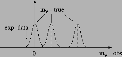
- Example 1:
- Measurement at the edge of a physical region.
An experiment, planned to measure the electron-neutrino mass
with a resolution of
 (independent of the
mass, for simplicity, see Fig. ),
finds a value of
(independent of the
mass, for simplicity, see Fig. ),
finds a value of
 (i.e.
this value comes out of the analysis of real data treated in exactly the same way as that
of simulated data, for which a
(i.e.
this value comes out of the analysis of real data treated in exactly the same way as that
of simulated data, for which a
 resolution was found).
What can we say about  ?
?
No physicist would sign a statement which sounded like he
was 98% sure of having found a negative mass!
Figure:
Negative neutrino mass?
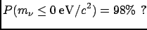 |
Figure:
Case of highly asymmetric expectation on the physics quantity.
 |
- Example 2:
- Non-flat distribution of a physical quantity.
Let us take a quantity that we know, from previous knowledge,
to be distributed as in
Fig. . It may be, for example,
the energy of bremsstrahlung photons
or of cosmic rays.
We know that an observable value 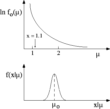 will be normally
distributed around the true value ,
independently of the value of . We have performed a
measurement and obtained
will be normally
distributed around the true value ,
independently of the value of . We have performed a
measurement and obtained  ,
in arbitrary units.
What can we say about the true value that has caused
this observation? Also in this case the formal definition
of the confidence interval does not work. Intuitively,
we feel that there is more chance that is on the left
side of (1.1) than on the right side. In the jargon of the experimentalists,
``there are more migrations from left
to right than from right to left''.
,
in arbitrary units.
What can we say about the true value that has caused
this observation? Also in this case the formal definition
of the confidence interval does not work. Intuitively,
we feel that there is more chance that is on the left
side of (1.1) than on the right side. In the jargon of the experimentalists,
``there are more migrations from left
to right than from right to left''.
- Example 3:
- High-momentum track in a magnetic spectrometer.
The previous examples deviate from the simple dog-hunter
picture only because of an asymmetric possible position of the `hunter'.
The case of a very-high-momentum track in a
central detector of a high-energy physics (HEP) experiment
involves asymmetric response of a detector for almost straight tracks
and non-uniform momentum distribution of charged particles produced
in the collisions. Also in this case the simple inversion scheme
does not work.
To sum up the last two sections, we can say that intuitive
inversion of probability
 |
(1.5) |
besides being theoretically unjustifiable,
yields results which are numerically correct only in the case
of symmetric problems.
Next: Misunderstandings caused by the
Up: Uncertainty in physics and
Previous: Probability of the causes
Contents
Giulio D'Agostini
2003-05-15