Caveat concerning the blind use of approximate methods

The mathematical apparatus of variances and covariances of ()-() is often seen as the most complete description of uncertainty and in most cases used blindly in further uncertainty calculations. It must be clear, however, that this is just an approximation based on linearization. If the function which relates the corrected value to the raw value and the systematic effects is not linear then the linearization may cause trouble. An interesting case is discussed in Section .

There is another problem which may arise from the simultaneous use of Bayesian estimators and approximate methods^6.5. Let us introduce the problem with an example.

Example 1:

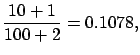
1000 independent measurements of the efficiency of a detector have been performed (or 1000 measurements of branching ratio, if you prefer). Each measurement was carried out on a base of 100 events and each time 10 favourable events were observed (this is obviously strange -- though not impossible -- but it simplifies the calculations). The result of each measurement will be (see ()-()):

$$\widehat{\epsilon}_i = \frac{10+1}{100+2} = 0.1078,$$ (6.19)

$$\sigma(\epsilon_i) = \sqrt{\frac{11\times 91}{103\times 102^2}} = 0.031\,.$$ (6.20)

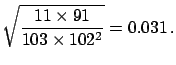
Combining the 1000 results using the standard weighted average procedure gives

$$\epsilon = 0.1078 \pm 0.0010\,.$$ (6.21)

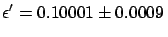
Alternatively, taking the complete set of results to be equivalent to 100 $$000 trials with 10 $$000 favourable events, the combined result is

$$\epsilon^\prime = 0.10001\pm 0.0009\,$$ (6.22)

(the same as if one had used Bayes' theorem iteratively to infer $f(\epsilon)$ from the the partial 1000 results). The conclusions are in disagreement and the first result is clearly mistaken (the solution will be given after the following example).

The same problem arises in the case of inference of the Poisson distribution parameter $\lambda$ and, in general, whenever 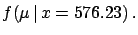$f(\mu)$ is not symmetrical around E$[\mu]$.

Example 2:

Imagine an experiment running continuously for one year, searching for monopoles and identifying none. The consistency with zero can be stated either quoting E$[\lambda]=1$ and $\sigma_\lambda=1$, or a $95\, \%$ upper limit $\lambda < 3$. In terms of rate (number of monopoles per day) the result would be either E$[r]=2.7\cdot 10^{-3}$, $\sigma(r)=2.7\cdot 10^{-3}$, or an upper limit $r<8.2\cdot 10^{-3}$. It is easy to show that, if we take the 365 results for each of the running days and combine them using the standard weighted average, we get $r=1.00\pm 0.05$ monopoles per day! This absurdity is not caused by the Bayesian method, but by the standard rules for combining the results (the weighted average formulae () and () are derived from the normal distribution hypothesis). Using Bayesian inference would have led to a consistent and reasonable result no matter how the 365 days of running had been subdivided for partial analysis.

This suggests that in some cases it could be preferable to give the result in terms of the value of $\mu$ which maximizes $f(\mu)$ ($p_m$ and $\lambda_m$ of Sections and ). This way of presenting the results is similar to that suggested by the maximum likelihood approach, with the difference that for $f(\mu)$ one should take the final probability density function and not simply the likelihood. Since it is practically impossible to summarize the outcome of an inference in only two numbers (best value and uncertainty), a description of the method used to evaluate them should be provided, except when $f(\mu)$ is approximately normally distributed (fortunately this happens most of the time).