Next: Poisson distributed quantities
Up: Counting experiments
Previous: Counting experiments
Contents
Binomially distributed observables
Let us assume we have performed  trials and obtained
  favourable events. What is the probability of the next event?
This situation happens frequently when measuring efficiencies,
branching ratios, etc. Stated more generally,
one tries to infer the ``constant
and unknown probability''5.6of an event occurring.
favourable events. What is the probability of the next event?
This situation happens frequently when measuring efficiencies,
branching ratios, etc. Stated more generally,
one tries to infer the ``constant
and unknown probability''5.6of an event occurring.
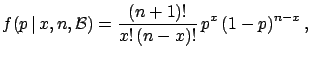
Where we can assume that the probability is constant
and the observed number of favourable events are binomially
distributed, the unknown quantity to be measured is the parameter
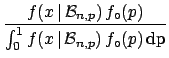
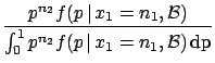
 of the binomial. Using Bayes' theorem we get
where an initial uniform distribution has been assumed.
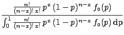
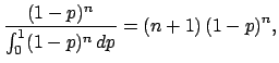
The final distribution is known to statisticians as  distribution
since the integral at the denominator is the special
function called , defined also for real values of and
(technically this is a with parameters
distribution
since the integral at the denominator is the special
function called , defined also for real values of and
(technically this is a with parameters
 and
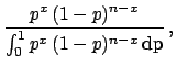
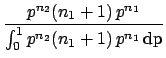
and  ). In our case
these two numbers are integer and the integral becomes
equal to
). In our case
these two numbers are integer and the integral becomes
equal to
 . We then get
 |
(5.32) |
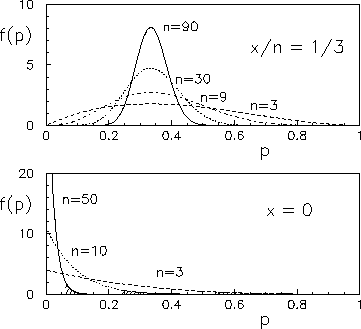
some example of which are shown in Fig. ![[*]](file:/usr/lib/latex2html/icons/crossref.png)
Figure:
Probability density function of the binomial parameter
, having observed successes in trials.
 |
The expectation value and the variance of this distribution
are:
E![$\displaystyle [p]$](img727.png) |
 |
 |
(5.33) |
Var |
|
 |
(5.34) |
| |
|
 |
|
| |
|
E![$\displaystyle [p]\,\left(1 - \mbox{E}[p]\right)\,\frac{1}{n+3}\,.$](img732.png) |
(5.35) |
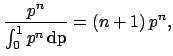
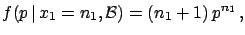
The value of for which  has the maximum is
instead
has the maximum is
instead  . The expression
E
. The expression
E![$ [p]$](img735.png) gives the prevision
of the probability for the
gives the prevision
of the probability for the  -th event
occurring and is called the
``recursive Laplace formula'', or ``Laplace's rule of succession''.
-th event
occurring and is called the
``recursive Laplace formula'', or ``Laplace's rule of succession''.
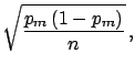
When and become large, and
 ,
has the following asymptotic properties:
,
has the following asymptotic properties:
| E |
 |
 |
(5.36) |
| Var |
|
 |
(5.37) |
 |
|
 |
(5.38) |
 |
 |
 |
(5.39) |
Under these conditions the frequentistic
``definition'' (evaluation rule!) of probability ( ) is recovered.
Let us see two particular situations: when  and
and  . In these
cases one gives the result as upper or lower limits, respectively.
Let us sketch the solutions:
. In these
cases one gives the result as upper or lower limits, respectively.
Let us sketch the solutions:
The following table shows the  probability limits as a function
of .
The Poisson approximation, to be discussed
in the next section, is also shown.
probability limits as a function
of .
The Poisson approximation, to be discussed
in the next section, is also shown.
| |
Probability level = |
|
|
|
| |
binomial |
binomial |
Poisson approx. |
| |
|
|
(
 ) ) |
| 3 |
 |
 |
 |
| 5 |
 |
 |
 |
| 10 |
 |
 |
 |
| 50 |
 |
 |
 |
| 100 |
 |
 |
 |
| 1000 |
 |
 |
|
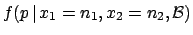
To show in this simple case how is updated by the new information,
let us imagine we have performed two experiments. The results
are  and
and  , respectively. Obviously the global
information
is equivalent to
, respectively. Obviously the global
information
is equivalent to  and
and  , with .
We then get
, with .
We then get
 |
(5.48) |
A different way of proceeding would have been to calculate the final
distribution from the information ,
 |
(5.49) |
and feed it as initial
distribution to the next inference:
getting the same result.
Next: Poisson distributed quantities
Up: Counting experiments
Previous: Counting experiments
Contents
Giulio D'Agostini
2003-05-15