


Next: BIPM and ISO recommendations
Up: Approximate methods
Previous: Approximate methods
Contents
Linearization
We have seen in the above examples how to use the
general formula (![[*]](file:/usr/lib/latex2html/icons/crossref.png) ) for practical applications.
Unfortunately,
when the problem becomes more complicated
one starts facing integration problems.
For this reason
approximate methods are generally used.
We will derive the approximation rules consistently
with the approach followed in these notes
and then the resulting formulae will
be compared with the ISO recommendations.
To do this, let us neglect for
a while all quantities of influence which could produce
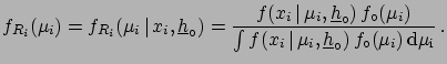
unknown systematic errors. In this case ()
can be replaced by (), which can be further simplified
if we remember that correlations between the results
are originated by unknown systematic errors. In the absence of these,
the joint distribution of all quantities
) for practical applications.
Unfortunately,
when the problem becomes more complicated
one starts facing integration problems.
For this reason
approximate methods are generally used.
We will derive the approximation rules consistently
with the approach followed in these notes
and then the resulting formulae will
be compared with the ISO recommendations.
To do this, let us neglect for
a while all quantities of influence which could produce
unknown systematic errors. In this case ()
can be replaced by (), which can be further simplified
if we remember that correlations between the results
are originated by unknown systematic errors. In the absence of these,
the joint distribution of all quantities
 is simply the product of
marginal ones:
is simply the product of
marginal ones:
 |
(6.1) |
with
 |
(6.2) |
The symbol
 indicates that we are dealing with
raw values6.1 evaluated at
indicates that we are dealing with
raw values6.1 evaluated at
 . Since for any variation
of
. Since for any variation
of
 the inferred values of
  will change,
it is convenient to name with the same subscript
will change,
it is convenient to name with the same subscript  the
quantity obtained for
the
quantity obtained for
 :
:
 |
(6.3) |
Let us indicate with
 and
and
 the best estimates and the standard uncertainty
of the raw values:
the best estimates and the standard uncertainty
of the raw values:
For any possible configuration of conditioning
hypotheses
, corrected values
are obtained:
 |
(6.6) |
The function which relates the corrected value to the raw value
and to the systematic effects has been denoted by  so as not to
be confused with a probability density function.
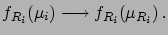
Expanding ()
in series around
we finally arrive at the expression
which will allow us to make the approximated
evaluations of uncertainties:
so as not to
be confused with a probability density function.
Expanding ()
in series around
we finally arrive at the expression
which will allow us to make the approximated
evaluations of uncertainties:
 |
(6.7) |
(All derivatives are evaluated at
 . To simplify
the notation a similar convention
will be used in the following formulae.)
. To simplify
the notation a similar convention
will be used in the following formulae.)
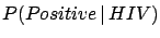
Neglecting the terms of the expansion above the first order,
and taking the expected values, we get
 |
 |
E![$\displaystyle [\mu_i]$](img613.png) |
|
| |
 |
 |
(6.8) |
 |
|
E![$\displaystyle \left[(\mu_i-\mbox{E}[\mu_i])^2\right]$](img921.png) |
|
| |
|
 |
|
| |
|
 |
(6.9) |
Cov |
|
E![$\displaystyle \left[\,(\mu_i-\mbox{E}[\mu_i])(\mu_j-
\mbox{E}[\mu_j])\,\right]$](img925.png) |
|
| |
|
 |
|
| |
|
 |
(6.10) |
The terms included within  vanish if the unknown systematic
errors are uncorrelated, and the formulae become simpler.
Unfortunately, very often this is not the
case, as when several calibration constants
are simultaneously obtained from a fit (for example, in most linear
fits slope and intercept have a correlation coefficient close to
vanish if the unknown systematic
errors are uncorrelated, and the formulae become simpler.
Unfortunately, very often this is not the
case, as when several calibration constants
are simultaneously obtained from a fit (for example, in most linear
fits slope and intercept have a correlation coefficient close to 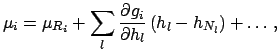 ).
).
Sometimes the expansion
() is not performed around the best values
of
but around their nominal
values, in the
sense that the correction for the known value of the systematic errors
has not yet been applied
(see Section ). In this case ()
should be replaced by
 |
(6.11) |
where the subscript  stands for nominal. The best value of
is then
stands for nominal. The best value of
is then
() and () instead remain valid,
with the condition that the derivative is calculated at
 .
If
.
If
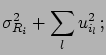 , it is possible to
rewrite () and ()
in the following way, which is very convenient for practical applications:
, it is possible to
rewrite () and ()
in the following way, which is very convenient for practical applications:
|
|
|
(6.13) |
| |
|
 |
(6.14) |
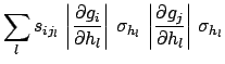
| Cov |
|
|
(6.15) |
| |
|
 |
(6.16) |
| |
|
 |
(6.17) |
| |
|
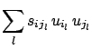
 Cov Cov |
(6.18) |
 is the component of the standard uncertainty due to effect
  .
.
 is equal to the product of signs of the derivatives,
which takes
into account whether the uncertainties are positively or negatively
correlated.
is equal to the product of signs of the derivatives,
which takes
into account whether the uncertainties are positively or negatively
correlated.
To summarize, when systematic effects are not correlated
with each other,
the following quantities are needed
to evaluate the corrected result, the
combined uncertainties and the correlations:
- the raw
and
;
- the best estimates of the corrections
 for each
systematic effect ;
for each
systematic effect ;
- the best estimate of the standard deviation due to the
imperfect knowledge of the systematic effect;
- for any pair
 the sign of the correlation
due to the effect .
the sign of the correlation
due to the effect .
In High Energy Physics applications it is frequently the case that
the derivatives appearing in
()-() cannot be calculated directly,
as for example when are parameters of a simulation program,
or acceptance cuts. Then variations of
 are
usually studied by varying a particular within
a reasonable interval, holding the other influence
quantities at the nominal value.
and are calculated from
the interval
are
usually studied by varying a particular within
a reasonable interval, holding the other influence
quantities at the nominal value.
and are calculated from
the interval
 of variation of the true value
for a given variation
of variation of the true value
for a given variation
 of
and from the probabilistic meaning of the intervals (i.e.
from the assumed distribution of the true value).
This empirical procedure for determining
and has the advantage that it
can take into account
non-linear effects[45], since it
directly measures the difference
of
and from the probabilistic meaning of the intervals (i.e.
from the assumed distribution of the true value).
This empirical procedure for determining
and has the advantage that it
can take into account
non-linear effects[45], since it
directly measures the difference
 for a given difference
 .
.
Some examples are given
in Section ,
and two typical experimental applications
will be discussed in more detail
in Section .
Next: BIPM and ISO recommendations
Up: Approximate methods
Previous: Approximate methods
Contents
Giulio D'Agostini
2003-05-15
 E
E![$\displaystyle \left[\sum_l \frac{\partial g_i}{\partial h_l}\,(h_l-h_{N_l})\right]$](img933.png)