Which generator?

Imagine two (pseudo-) random number generators: $H_1$, Gaussian with mean 0 and standard deviation 1, and $H_2$, also Gaussian, but with mean 0.4 and standard deviation 2 (see figure 9).

A program chooses at random, with equal probability, $H_1$ or $H_2$; then the generator produces a number, that, rounded to the 7-th decimal digit, is $x_E=0.3986964$. The question is, from which random generator does $x_E$ come from?

At this point, the problem is rather easy to solve, if we know the probability of each generator to give $x_E$. They are⁵⁴

$$P(x_E\,\vert\,H_1,I) = 3.68\times 10^{-8} \ \ \ ( \mbox{1 in $\approx$\,27 millions} )$$

$$P(x_E\,\vert\,H_2,I) = 1.99\times 10^{-8} \ \ \ ( \mbox{1 in $\approx$\,50 millions} )\,,$$

from which we can calculate Bayes factor and weight of evidence:

$$\begin{array}{rclcl} \tilde O_{1,2}(x_E,I) &=& 1.85 \ \ \ &\Rightarrow& \Delta\mbox{JL}_{1,2}(x_E,I) = +0.27\,. \end{array}$$

Therefore, the observation of $x_E$ provides a slight evidence in favor of $H_1$, no matter if this generator has very little probability to give $x_E$, as it has very little probability to give any particular number.

Figure: Which random number generator has produced $x_E$? Which hypothesis favors the points indicated by `$\times$'?

What matters when comparing hypotheses is never, stated in general terms, the absolute probability $P(E\,\vert\,H_i,I)$. 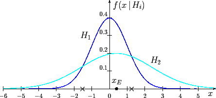In particular, it doesn't make sense saying `` $P(H_i\,\vert\,E,I)$ is small because $P(E\,\vert\,H_i,I)$ is small''.⁵⁵ As a consequence, from a consistent probabilistic point of view, it makes no sense to test a single, isolated hypothesis, using `funny arguments', like how far if $x_E$ from the peak of $f(x\,\vert\,H_i)$, or how large is the area below $f(x\,\vert\,H_i)$ from $x=x_E$ to infinity. In particular, if two models give exactly the same probability to produce an observation, like the two points indicated by `$\times$' in fig. 9, the evidence provided by this observation is absolutely irrelevant [ $\Delta$JL$_{1,2}($`$\times$'$)=0$].

To get a bit familiar with the weight of evidence in favor of either hypothesis provided by different observations, the following table, reporting Bayes factors and JL's due to the integers between $-6$ and $+6$, might be useful.

$x_E$		$\tilde O_{1,2}(x_E)$	$\Delta$JL $_{1,2}(x_E)$
$-6$		$5.1\times 10^{-6}$	$-5.3$
$-5$		$2.9\times 10^{-4}$	$-3.5$
$-4$		$7.5\times 10^{-3}$	$-2.1$
$-3$		$9.4\times 10^{-2}$	$-1.0$
$-2$		$0.56$	$-0.3$
$-1$		$1.5$	$0.2$
0		$2.0$	$0.3$
$1$		$1.3$	$0.1$
$2$		$0.37$	$-0.4$
$3$		$5.2\times 10^{-2}$	$-1.3$
$4$		$3.4\times 10^{-3}$	$-2.5$
$5$		$1.0\times 10^{-4}$	$-4.0$
$6$		$1.5\times 10^{-6}$	$-5.8$

As we see from this table, and as we better understand from figure 9, numbers large in module are in favor of $H_2$, and very large ones are in its strong favor. Instead, the numbers laying in the interval defined by the two points marked in the figure by a cross provide evidence in favor of $H_1$. However, while individual pieces of evidence in favor of $H_1$ can only be weak (the maximum of $\Delta$JL is about 0.3, reached around $x=0$, namely $-0.13$, to be precise, for which $\Delta$JL reaches 0.313), those in favor of the alternative hypothesis can be sometimes very large. It follows then that one gets easier convinced of $H_2$ rather than of $H_1$.

We can check this by a little simulation. We choose a model, extract 50 random variables and analyze the data as if we didn't know which generator produced them, although considering $H_1$ and $H_2$ equally likely. We expect that, as we go on with the extractions, the pieces of evidence accumulate until we possibly reach a level of practical certainty. Obviously, the individual pieces of evidence do not provide the same $\Delta$JL, and also the sign can fluctuate, although we expect more positive contributions if the points are generated by $H_1$ and the other way around if they came from $H_2$. Therefore, as a function of the number of extractions the accumulated weight of evidence follows a kind of asymmetric random walk (imagine the JL indicator fluctuating as the simulated experiment goes on, but drifting `in average' in one direction).

Figure: Combined weights of evidence in simulated experiments. The above (blue) combined JL sequences have been obtained by the generator $H_1$, as it can be recognized because they tend to large positive values as the number of extractions increases. The below one are generated by $H_2$.

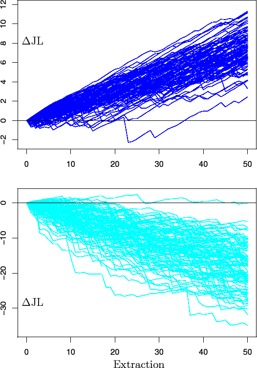Figure 10 shows 200 inferential stories, half per generator. We see that, in general, we get practically sure of the model after a couple of dozens of extractions. But there are also cases in which we need to wait longer before we can feel enough sure on one hypothesis.

It is interesting to remark that the leaning in favor of each hypothesis grows, in average, linearly with the number of extractions. That is, a little piece of evidence, which is in average positive for $H_1$ and negative for $H_2$, is added after each extraction. However, around the average trend, there is a large varieties of individual inferential histories. They all start at $\Delta$JL$=0$ for $n=0$, but in practice there are no two identical `trajectories'. All together they form a kind of `fuzzy band', whose `effective width' grows also with the number of extractions, but not linearly. The widths grows as the square root of $n$.<sup>56</sup>This is the reason why, as $n$ increases, the bands tend to move away from the line JL$=0$. Nevertheless, individual trajectories can exhibit very `irregular'⁵⁷ behaviors as we can also see in figure 10.