In most cases (and practically always in courts)
pieces of evidence are not acquired directly by the person
who has to form his mind about the plausibility of a hypothesis.
They are usually accounted by an intermediate person, or
by a chain of individuals.
Let us call  the report of the
evidence
the report of the
evidence  provided in a testimony.
The inference becomes now
provided in a testimony.
The inference becomes now
 , generally
different from
, generally
different from
 .
.
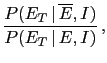
In order to apply Bayes' theorem in one of its form
we need first to evaluate
 .
Probability theory teaches us how to get it
[see Eq. (33) in Appendix A]:
.
Probability theory teaches us how to get it
[see Eq. (33) in Appendix A]:
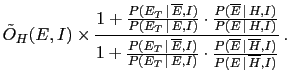
( could be due to a true evidence or to a fake one).
Three new ingredients enter the game:
-
 , that is the probability of
the evidence to be correctly reported as such.
, that is the probability of
the evidence to be correctly reported as such.
- But the testimony could also be incorrect the other way around
(it could be incorrectly reported, simply by mistake,
but also it could be a `fabricated evidence'),
and therefore also
 is needed.
Note that the probabilities to lie could be in general
asymmetric, i.e.
is needed.
Note that the probabilities to lie could be in general
asymmetric, i.e.
 ,
as we have seen in the AIDS problem of Appendix F, in which
the response of the analysis models false witness well.
,
as we have seen in the AIDS problem of Appendix F, in which
the response of the analysis models false witness well.
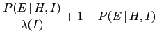
- Finally, since
 enters now directly,
the `naïve' Bayes factor, only depending
on
enters now directly,
the `naïve' Bayes factor, only depending
on
 , is not longer enough.
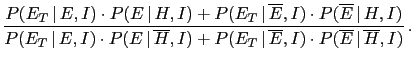
Taking our usual two hypotheses,
 `guilty'
and
`guilty'
and
 `innocent', we get the following
Bayes factor based on the testified evidence
(hereafter, in order to simplify the notation,
we use the subscript `
`innocent', we get the following
Bayes factor based on the testified evidence
(hereafter, in order to simplify the notation,
we use the subscript ` ' in odds and Bayes factors,
instead of `
' in odds and Bayes factors,
instead of ` ',
to indicate that they are in favor of and against
',
to indicate that they are in favor of and against
 ,
as we already did in the
AIDS example of Appendix F):
,
as we already did in the
AIDS example of Appendix F):
As expected, this formula is a bit more complicate that the
Bayes factor calculated taking for granted, which is recovered
if the lie probabilities vanish
i.e. only when
we are absolutely sure the witness does not
err or lie reporting
(but Peirce reminds us that ``absolute certainty,
or an infinite chance, can never be attained by
mortals'' [6]).
In order to single out the effects of the new ingredients, Eq. (39)
can be rewritten as62
where
under the condition63
 and
and
 , i.e.
 positive and finite.
The parameter
positive and finite.
The parameter
 , ratio of the probability of fake evidence and the
probability that the evidence is correctly accounted,
can be interpreted as a kind of lie factor.
Given the human roughly logarithmic sensibility to probability
ratios, it might be useful to define, in analogy to the JL,
, ratio of the probability of fake evidence and the
probability that the evidence is correctly accounted,
can be interpreted as a kind of lie factor.
Given the human roughly logarithmic sensibility to probability
ratios, it might be useful to define, in analogy to the JL,
Let us make some instructive limits of Eq. (41).
As we have seen, the ideal case is recovered if the lie factor vanishes.
Instead, if it is equal to 1, i.e.
J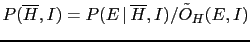 , the reported
evidence becomes useless. The same happens if
, the reported
evidence becomes useless. The same happens if
 vanishes
[this implies that
vanishes
[this implies that
 vanishes too, being
 ].
].
However, the most remarkable limit
is the last one. It states
that, even if
is very high,
the effective Bayes factor cannot exceed the inverse of the lie factor:
or, using logarithmic quantities
At this point some numerical examples are in order (and those
who claim they can form their mind on pure intuition
get all my admiration...if they really can).
Let us imagine that would ideally provide a weight of evidence
of 6 [i.e.
 JL
JL ]. We can study, with the help
of table 2,
]. We can study, with the help
of table 2,
Table:
Dependence
of the judgement leaning due to a reported evidence
[
JL ] for
JL, 3 and 1
as a function the other ingredients of the inference
(see text). Note the upper
limit of
JL to
] for
JL, 3 and 1
as a function the other ingredients of the inference
(see text). Note the upper
limit of
JL to
 J
J , if this value is
 JL
JL .
.
|
|
JL |
|
J |
|
JL |
| |
JL : : |
10 |
 |
 |
 |
0 |
 |
 |
 |
 |
|
6.00 |
6.00 |
6.00 |
6.00 |
6.00 |
6.00 |
6.00 |
6.00 |
 |
|
6.00 |
6.00 |
6.00 |
6.00 |
5.99 |
5.95 |
4.96 |
 |
 |
|
5.96 |
5.96 |
5.96 |
5.95 |
5.92 |
5.68 |
4.00 |
 |
 |
|
5.70 |
5.70 |
5.70 |
5.68 |
5.52 |
4.92 |
3.00 |
 |
 |
|
4.96 |
4.96 |
4.95 |
4.92 |
4.68 |
3.95 |
2.00 |
 |
 |
|
4.00 |
4.00 |
3.99 |
3.95 |
3.70 |
2.96 |
1.04 |
 |
|
|
3.00 |
3.00 |
3.00 |
2.96 |
2.70 |
1.96 |
0.30 |
 |
 |
|
2.00 |
2.00 |
2.00 |
1.95 |
1.70 |
1.00 |
0.04 |
 |
|
|
1.00 |
1.00 |
1.00 |
0.96 |
0.74 |
0.26 |
0.004 |
 |
| 0 |
|
0 |
0 |
0 |
0 |
0 |
0 |
0 |
0 |
|
JL |
|
J |
|
JL |
| |
JL: |
10 |
|
|
|
0 |
|
|
|
|
|
|
3.00 |
3.00 |
3.00 |
3.00 |
3.00 |
3.00 |
3.00 |
3.00 |
|
|
3.00 |
3.00 |
3.00 |
3.00 |
2.99 |
2.95 |
1.96 |
|
|
|
2.96 |
2.96 |
2.96 |
2.95 |
2.92 |
2.68 |
1.04 |
|
|
|
2.70 |
2.70 |
2.70 |
2.68 |
2.52 |
1.93 |
0.30 |
|
|
|
1.96 |
1.96 |
1.96 |
1.92 |
1.68 |
1.00 |
0.04 |
|
|
|
1.00 |
1.00 |
0.99 |
0.96 |
0.74 |
0.26 |
0.004 |
|
| 0 |
|
0 |
0 |
0 |
0 |
0 |
0 |
0 |
0 |
|
JL |
|
J |
|
JL |
| |
JL: |
10 |
|
|
|
0 |
|
|
|
|
|
|
1.00 |
1.00 |
1.00 |
1.00 |
1.00 |
1.00 |
1.00 |
1.00 |
|
|
1.00 |
1.00 |
1.00 |
1.00 |
0.99 |
0.96 |
0.26 |
|
|
|
0.96 |
0.96 |
0.96 |
0.96 |
0.93 |
0.72 |
0.04 |
|
|
|
0.72 |
0.72 |
0.72 |
0.70 |
0.58 |
0.23 |
0.003 |
|
 |
|
0.41 |
0.41 |
0.41 |
0.39 |
0.27 |
0.07 |
 |
|
| 0 |
|
0 |
0 |
0 |
0 |
0 |
0 |
0 |
0 |
|
how the weight of the reported evidence
JL
depends on the other beliefs [in this table logarithmic
quantities have been used throughout, therefore
JL is the base ten logarithm of the odds in favor
of given the hypothesis ; the table provides, for comparisons,
also
JL from
JL equal to 3 and 1].
is the base ten logarithm of the odds in favor
of given the hypothesis ; the table provides, for comparisons,
also
JL from
JL equal to 3 and 1].
The table exhibits the limit behaviors we have seen analytically.
In particular,
if we fully trust the report, i.e.
J ,
then
JL is exactly equal to
JL
,
then
JL is exactly equal to
JL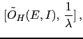 ,
as we already know. But as soon as the absolute value of the lie factor
is close to
JL, there is a sizeable effect.
The upper bound can be the be rewritten as
,
as we already know. But as soon as the absolute value of the lie factor
is close to
JL, there is a sizeable effect.
The upper bound can be the be rewritten as
 |
 |
min![$\displaystyle \,
[\tilde O_{H}(E,I),\, \frac{1}{\lambda}]\,,$](img530.png) |
(50) |
| or |
|
|
|
 JL JL |
|
min JL JL J J![$\displaystyle \lambda(I)] \,,$](img534.png) |
(51) |
a relation valid in the region of interest when thinking
about an evidence in favor of , i.e.
JL and
J
and
J .
.
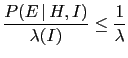
This upper bound is very interesting. Since minimum conceivable values
of
J for human beings can be of the order of
(to perhaps
 or
or
 ,
but in many practical applications or can already be very generous!),
in practice the effective weights of evidence cannot exceed
values of about
,
but in many practical applications or can already be very generous!),
in practice the effective weights of evidence cannot exceed
values of about  (I have no strong opinion on the exact
value of this limit, my main point is that you consider
there might be
such a practical human limit.)
(I have no strong opinion on the exact
value of this limit, my main point is that you consider
there might be
such a practical human limit.)
This observation has an important consequence in the combination of evidences,
as anticipated at the end of section 3.5.
Should we give more consideration to
a single strong piece of evidence, virtually weighing
JL , or 10 independent weaker evidences,
each having a JL of 1? As it was said, in the ideal case
they yield the same global leaning factor.
But as soon as human fallacy (or conspiracy) is taken into account,
and we remember that our belief is based on and not on ,
then we realize that
JL
, or 10 independent weaker evidences,
each having a JL of 1? As it was said, in the ideal case
they yield the same global leaning factor.
But as soon as human fallacy (or conspiracy) is taken into account,
and we remember that our belief is based on and not on ,
then we realize that
JL is well above the range
of JL that we can reasonably conceive.
Instead the weaker pieces of evidence are little affected
by this doubt and when they sum up together, they really
can provide a JL of about 10.
is well above the range
of JL that we can reasonably conceive.
Instead the weaker pieces of evidence are little affected
by this doubt and when they sum up together, they really
can provide a JL of about 10.
Giulio D'Agostini
2010-09-30