Extra variability of the data

As clearly stated, the previous results assume that the only sources of deviation of the measurements from the value of the physical quantities are normal errors, with known standard deviations $\sigma_{x_i}$ and $\sigma_{y_i}$ . Sometimes, as it is the case of the data points reported in Ref. [14], this is not the case. This means that $y$ depends also on other, `hidden' variables, and what we observe is the overall effects integrated over all the variability of the variables that we do not `see'. In lack of more detailed information, the simplest modification to the model described above is to add an extra Gaussian `noise' on one of the coordinates. For tradition and simplicity this extra noise is added to the $y$ variable. The effect on the above result can be easily understood. Let us call $\sigma _v$ the r.m.s. of this extra noise that acts normally and independently in each $y$ point. As it is well known, the sum of Gaussian distributions is still Gaussian with an expected value and variance respectively sum of the individual expected values and variances. Therefore, the effect in the individual likelihoods (28) is to replace $\sigma^2_{y_i}$ by $\sigma^2_{y_i}+\sigma^2_v$. But we now have an extra parameter in the model, and Eq. (30) becomes

$$f(m,c,\sigma_v\,\vert\,{\mbox{\boldmath$x$}},{\mbox{\boldmath$y$}},I) \propto \prod_i \frac{1}{\sqrt{\sigma^2_v + \sigma_{y_i}^2+m^2\,\sigma_{x... ...+ \sigma_{y_i}^2+m^2\,\sigma_{x_i}^2) } \right]}\, f(m,c,\sigma_v\,\vert\,I)\,.$$

More rigorously, this formula can be obtained from a variation of reasoning followed in the previous section.

• $\mu_y$ depends on $\mu_x$ and on the set of hidden variables ${\mbox{\boldmath$v$}}$:
  

  $$\mu_y = \mu_y^{(v)}(\mu_x,{\mbox{\boldmath$\theta$}}, {\mbox{\boldmath$v$}})$$ (35)

  $$= z(\mu_x,{\mbox{\boldmath$\theta$}}) + g(\mu_x,{\mbox{\boldmath$v$}})\,$$ (36)

  
  
  where the overall dependence $\mu_y^{(v)}(\,\,)$ has been split in two functions: $z(\mu_x,{\mbox{\boldmath$\theta$}})$, only depending on $\mu_x$ and the model parameters, corresponding to the ideal case; $g(\mu_x,{\mbox{\boldmath$v$}})$ describing the difference from the ideal case.
• Calling $z$ the fictitious variable, deterministically dependent on $\mu_x$, for a given $\mu_{x_i}$ we have the following model
  

  $$z_i = z(\mu_{x_i}, {\mbox{\boldmath$\theta$}}) \,: f(z_i\,\vert\,\mu_{x_i}, {\mbox{\boldmath$\theta$}},I) = \delta[\,z_i - z(\mu_{x_i},{\mbox{\boldmath$\theta$}})\,]$$ (37)

  $$\mu_{y_i} \,: f(\mu_{y_i}\,\vert\,z_i,I)\,$$ (38)

  
  
  where $f(\mu_{y_i}\,\vert\,z_i,I)$ describes our uncertainty about $\mu_{y_i}$ due to the unknown values of all other hidden variables.
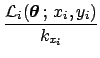
• We need now to specify $f(\mu_{y_i}\,\vert\,z_i,I)$. As usual, in lack of better knowledge, we take a Gaussian distribution of unknown parameter $\sigma _v$, with awareness that this is just a convenient, approximated way to quantify our uncertainty.

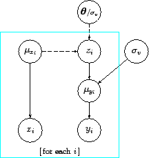
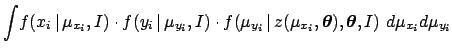
  At this point a summary of all ingredients of the model in the specific case of linear model is in order:
  

  $$y_i \sim {\cal N}(\mu_{y_i}, \sigma_{y_i})$$ (39)

  $$x_i \sim {\cal N}(\mu_{x_i}, \sigma_{x_i})$$ (40)

  $$z_i \leftarrow m\, \mu_{x_i} + c \hspace{10.0mm} [\,\Rightarrow\ \delta(z_i- m\, \mu_{x_i} + c)\,]$$ (41)

  $$\mu_{y_i} \sim {\cal N}(z_i, \sigma_{v})$$ (42)

  $$\mu_{x_i} \sim {\cal U}(-\infty,+\infty) \hspace{5.0mm} [\,\Rightarrow\ k_{x_i}\,]$$ (43)

  $$m,c,\sigma_v \Rightarrow \mbox{see later} \hspace{12.4mm} [\,\Rightarrow \mbox{'uniform'}\,],$$ (44)

  
  
  where ${\cal U}(-\infty,+\infty)$ stands for a uniform distribution over a very large interval, and the symbol `$\leftarrow$' has been used to deterministically assign a value, as done in BUGS[11] (see later).
• We have now the extra parameter $\sigma _v$ that we include in ${\mbox{\boldmath$\theta$}}$, so that $M$ increases by 1. The new model in represented in Fig. 2,

  Figure: Minimal modification of Fig. 1 to model the extra variability not described by the error functions. Note that ${\mbox{\boldmath$\theta$}}$ stands for all model parameters to be inferred, including $\sigma _v$. Instead, ${\mbox{\boldmath$\theta$}}/\sigma_v$ stands for all parameters apart from $\sigma _v$.

  
  in which we have indicated by ${\mbox{\boldmath$\theta$}}/\sigma_v$ all parameters apart from $\sigma _v$.
• The variables of the model are now $5 N+M$, and Eq. (22) becomes
  

  $$f({\mbox{\boldmath$x$}},{\mbox{\boldmath$y$}},{\mbox{\boldmath$\m... ...{\boldmath$\mu$}}_y,{\mbox{\boldmath$z$}},{\mbox{\boldmath$\theta$}}\,\vert\,I) \propto \prod_i f(x_i\,\vert\,\mu_{x_i},I) \cdot f(y_i\,\vert\,\mu_{\mu_i},I)$$

  $$\ \ \ \cdot f(\mu_{y_i}\,\vert\,z_i,I) \cdot\, \delta[\,z_i - z(\... ...box{\boldmath$\theta$}})\,]\, \cdot f({\mbox{\boldmath$\theta$}}\,\vert\,I) \,.$$ (45)

  
  

• Consequently, Eq. (10) becomes
  

  $$f({\mbox{\boldmath$\theta$}}\,\vert\,{\mbox{\boldmath$x$}},{\mbox{\boldmath$y$}},I) \propto \int\! f({\mbox{\boldmath$x$}},{\mbox{\boldmath$y$}},{\mbox{\bold... ...\mbox{\boldmath$\mu$}}_x\,d{\mbox{\boldmath$\mu$}}_y\,d{\mbox{\boldmath$z$}}\,.$$ (46)

  
  

• Inserting the model functions (40)-(45) in Eq. (46), after the marginalization (47) and the factorization of the result into likelihood as prior [as previously done in (24)], we get the analogues of Eqs. (26)-(28):
  

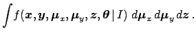
  $$\frac{{\cal L}_i({\mbox{\boldmath$\theta$}}\,;\,x_i,y_i)}{k_{x_i}} = \int\! f(x_i\,\vert\,\mu_{x_i},I) \cdot f(y_i\,\vert\,\mu_{y_i},I... ... z(\mu_{x_i},{\mbox{\boldmath$\theta$}})\,] \,\, d{\mu_{x_i}}d{\mu_{y_i}}d{z_i}$$ (47)

  $$= \int\! f(x_i\,\vert\,\mu_{x_i},I) \cdot f(y_i\,\vert\,\mu_{y_i},I... ...ox{\boldmath$\theta$}}),{\mbox{\boldmath$\theta$}},I) \,\, d\mu_{x_i}d\mu_{y_i}$$ (48)

  $$= \int \frac{1}{\sqrt{2\pi}\, \sigma_{x_i}}\, \exp{ \left[ -\frac{(... ...a_{y_i}}\, \exp{ \left[ -\frac{(y_i-\mu_{y_i})^2} {2\,\sigma_{y_i}^2} \right] }$$

  $$\hspace{3.0mm}\cdot \frac{1}{\sqrt{2\pi}\, \sigma_{v}}\, \exp{ \l... ..._i}-m\,\mu_{x_i}-c)^2} {2\,\sigma_{v}^2} \right] } \,\, d\mu_{x_i} d\mu_{y_i}\,$$ (49)

  $$= \int \frac{1}{\sqrt{2\pi}\, \sigma_{x_i}}\, \exp{ \left[ -\frac{(x_i-\mu_{x_i})^2} {2\,\sigma_{x_i}^2} \right] }$$

  $$\hspace{3.0mm} \cdot \frac{1}{\sqrt{2\pi}\, \sqrt{\sigma_{v}^2+\s... ...\mu_{x_i}-c)^2} {2\,(\sigma_{v}^2+\sigma_{y_i}^2)} \right] } \,\, d\mu_{x_i} \,$$ (50)

  $$= \frac{1}{\sqrt{2\pi}\, \sqrt{\sigma_{v}^2+\sigma_{y_i}^2 +m^2\sig... ..._i}-m\,x_i-c)^2} {2\,(\sigma_{v}^2+\sigma_{y_i}^2+m^2\sigma_{x_i}^2)} \right] }$$ (51)

  
  

• Inserting in Eq. (25) the expression of ${\cal L}_i({\mbox{\boldmath$\theta$}}\,;\,x_i,y_i)$ coming from Eq. (52) we get finally Eq. (35).