


Next:
Up: Partial results from ,
Previous: Partial results from ,

Applying our reasoning to the constraint given by
, we obtain
The contour plot shown in Fig. 1 for
 .
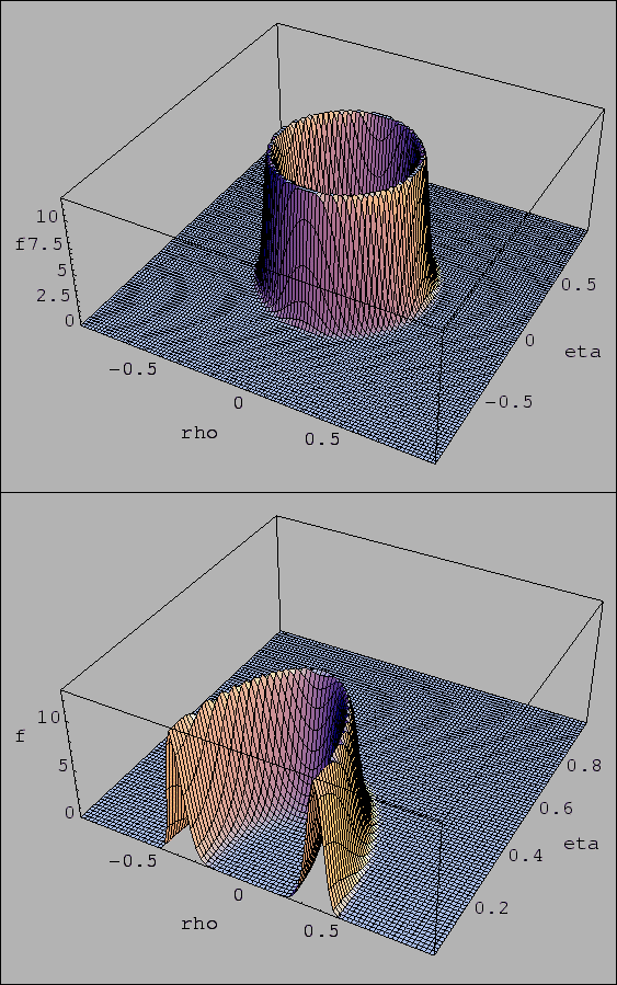
3-D plots are given in Fig. 2 (in all figures
``rho'' and ``eta'' stand for
.
3-D plots are given in Fig. 2 (in all figures
``rho'' and ``eta'' stand for  and
and  ).
).
Figure:
Contour plot of the p.d.f. of Fig. 2 for
. Note that contours are simply iso-p.d.f. levels obtained
by 12 contour lines. In order to assign them a probabilistic meaning,
one needs to evaluate the p.d.f. integrals inside the contours.
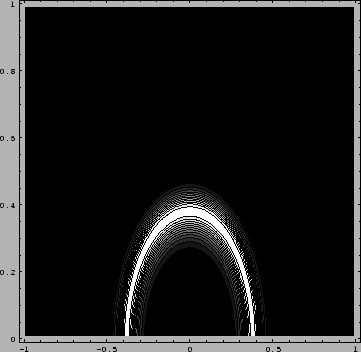 |
Figure:
Probability density function of and
obtained by the constraint given by
.
 |
Note that the plot of Fig. 1 is obtained slicing
 into 12 iso-p.d.f. contours, and hence
the regions shown there have no straightforward
probabilistic interpretation,
since one should make the integrals of the p.d.f. inside the region.
We leave it as an exercise for the interested readers.
into 12 iso-p.d.f. contours, and hence
the regions shown there have no straightforward
probabilistic interpretation,
since one should make the integrals of the p.d.f. inside the region.
We leave it as an exercise for the interested readers.
Next:
Up: Partial results from ,
Previous: Partial results from ,
Giulio D'Agostini
2004-01-20
![$\displaystyle \int_{-\infty}^{+\infty}\!
\delta(\bar {\rho}^2+\bar{\eta}^2-a)\,...
...\pi}\,0.031}\,
\exp{\left[-\frac{(a-0.145)^2}{2\,(0.031)^2}\right]}\, \mbox{d}a$](img63.png)
![$\displaystyle \frac{1}{\sqrt{2\,\pi}\,0.031}\,
\exp{\left[-\frac{(\bar {\rho}^2+\bar{\eta}^2-0.145)^2}{2\,(0.031)^2}\right]}\,.$](img64.png)