


Next: A probabilistic theory of
Up: Uncertainty in physics and
Previous: Misunderstandings caused by the
Contents
Statistical significance versus probability of hypotheses
The examples in the previous
section have shown the typical ways in which significance tests
are misinterpreted.
This kind of mistake is commonly made
not only by students, but also by professional users of statistical
methods. There are two different probabilities:
-
 :
:
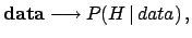
- the probability of the
hypothesis
 , conditioned by the observed data.
This is the probabilistic statement in which
we are interested. It summarizes the status of
knowledge on , achieved in conditions of uncertainty: it
might be the probability that the
, conditioned by the observed data.
This is the probabilistic statement in which
we are interested. It summarizes the status of
knowledge on , achieved in conditions of uncertainty: it
might be the probability that the  mass is between
80.00 and 80.50 GeV, that the Higgs mass is below 200 GeV,
or that a charged track is a
mass is between
80.00 and 80.50 GeV, that the Higgs mass is below 200 GeV,
or that a charged track is a  rather than a
  .
.
-
 :
:
- the probability of the observables
under the condition that the hypothesis is
true.1.14
For example,
the probability of getting two consecutive heads when
tossing a regular coin, the probability
that a mass is reconstructed
within 1 GeV of the true mass,
or that a 2.5 GeV pion produces a
 pC signal in
an electromagnetic calorimeter.
pC signal in
an electromagnetic calorimeter.
Unfortunately, conventional statistics considers only the
second case. As a consequence,
since the very question of interest remains unanswered,
very often
significance levels
are incorrectly treated as if they were
probabilities of the hypothesis.
For example, `` refused at 5% significance''
may be understood to mean the same as `` has only 5%
probability of being true.''
It is important to note the different
consequences of the misunderstanding caused by
the arbitrary probabilistic interpretation of
confidence intervals and of significance levels.
Measurement uncertainties on directly measured quantities
obtained by confidence intervals
are at least numerically correct in most routine cases,
although arbitrarily interpreted.
In hypothesis tests, however,
the conclusions
may become seriously wrong. This can be shown with the following
examples.
- Example 7:
- AIDS test.
An Italian citizen is chosen at random to undergo an AIDS test. Let us assume
that the analysis used to test for HIV infection has the following
performances:
The analysis may declare healthy people `Positive', even if only
with a very small probability.
Let us assume that the analysis states `Positive'.
Can we say that, since the probability
of an analysis error Healthy
 Positive is only
  ,
then the probability that the person is infected is
,
then the probability that the person is infected is  ?
Certainly not. If one calculates on the basis
of an estimated 100000 infected
persons out of a population of
?
Certainly not. If one calculates on the basis
of an estimated 100000 infected
persons out of a population of  million, there is a
 probability that the person is healthy!1.15
Some readers may be surprised to read that, in order to reach a
conclusion, one needs to have an idea of how `reasonable'
the hypothesis is, independently of the data used: a mass cannot
be negative; the spectrum of the true value is of a certain type;
students often make mistakes; physical hypotheses happen to be
incorrect; the proportion of Italians carrying the HIV virus is roughly
probability that the person is healthy!1.15
Some readers may be surprised to read that, in order to reach a
conclusion, one needs to have an idea of how `reasonable'
the hypothesis is, independently of the data used: a mass cannot
be negative; the spectrum of the true value is of a certain type;
students often make mistakes; physical hypotheses happen to be
incorrect; the proportion of Italians carrying the HIV virus is roughly
 in
in  . The notion of prior reasonableness of the hypothesis
is fundamental to the approach we are going to present, but
it is something to which
physicists put up strong resistance (although in practice they
often instinctively use this intuitive way of reasoning continuously
and correctly). In this report
I will try to show that `priors' are rational and unavoidable,
although their influence may become negligible when there is
strong experimental evidence in favour of a given hypothesis.
. The notion of prior reasonableness of the hypothesis
is fundamental to the approach we are going to present, but
it is something to which
physicists put up strong resistance (although in practice they
often instinctively use this intuitive way of reasoning continuously
and correctly). In this report
I will try to show that `priors' are rational and unavoidable,
although their influence may become negligible when there is
strong experimental evidence in favour of a given hypothesis.
- Example 8:
- Probabilistic statements about the 1997 HERA high-
 events.
A very instructive example of the misinterpretation of probability
can be found in the statements which commented on the
excess of events observed by the HERA experiments at
DESY in the high- region.
For example, the official DESY statement [13]
was:1.16
``The two HERA experiments, H1 and ZEUS,
observe an excess of events above
expectations at
high  (or
(or
 ),
),  , and .
For
, and .
For

 the joint
distribution has a probability of less than one per cent to come
from Standard Model NC DIS processes.''
Similar statements were spread out in the scientific community,
and finally to the press. For example,
a message circulated by INFN stated
(it can be understood even in Italian)
the joint
distribution has a probability of less than one per cent to come
from Standard Model NC DIS processes.''
Similar statements were spread out in the scientific community,
and finally to the press. For example,
a message circulated by INFN stated
(it can be understood even in Italian)
``La probabilità che gli eventi osservati siano una fluttuazione
statistica è inferiore all' 1%.''
Obviously these two statements led the press
(e.g. Corriere della Sera, 23 Feb. 1998) to announce that
scientists were highly confident that a great discovery
was just around the corner.1.17
The experiments, on the other hand, did not mention this
probability. Their published results[15]
can be summarized, more or less, as
``there is a
 probability
of observing such
events or rarer ones within the Standard Model''.
probability
of observing such
events or rarer ones within the Standard Model''.
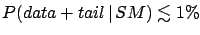
To sketch the flow of consecutive statements, let us
indicate by
 ``the Standard Model is
the only cause which can produce these events'' and by
tail the ``possible observations which are rarer
than the configuration of data actually observed''.
``the Standard Model is
the only cause which can produce these events'' and by
tail the ``possible observations which are rarer
than the configuration of data actually observed''.
- Experimental result:
 .
.
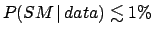
- Official statements:
 .
.
- Press:
 ,
simply applying standard logic to the outcome of step 2.
They deduce, correctly, that the hypothesis
,
simply applying standard logic to the outcome of step 2.
They deduce, correctly, that the hypothesis
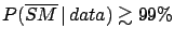 (= hint of new physics) is almost certain.
One can recognize an arbitrary inversion of probability. But now there is
also something else, which is more subtle,
and suspicious: ``why should we also
take into account data which have not been
observed?''1.18
Stated in a schematic way,
it seems natural to draw conclusions
on the basis of the observed data:
although
 differs from
 .
But it appears strange that unobserved data too should play
a role. Nevertheless, because of our educational background,
we are so used to the inferential scheme of the kind
that we even have difficulty in understanding the meaning of this
objection.1.19
.
But it appears strange that unobserved data too should play
a role. Nevertheless, because of our educational background,
we are so used to the inferential scheme of the kind
that we even have difficulty in understanding the meaning of this
objection.1.19
Let us consider a new case, conceptually very similar, but easier
to understand intuitively.
- Example 9:
- Probability that a particular random number
comes from a generator.
The value 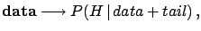 is extracted from a Gaussian random-number
generator having
is extracted from a Gaussian random-number
generator having
 and
and  . It is well known that
but we cannot state that
the value has 0.27% probability
of coming from that generator, or that the probability that the
observation is a statistical fluctuation is 0.27%.
In this case, the value comes with 100% probability from
that generator, and it is at 100% a statistical fluctuation.
This example helps to illustrate the logical mistake one can make
in the previous examples. One may speak about the probability of the
generator (let us call it
. It is well known that
but we cannot state that
the value has 0.27% probability
of coming from that generator, or that the probability that the
observation is a statistical fluctuation is 0.27%.
In this case, the value comes with 100% probability from
that generator, and it is at 100% a statistical fluctuation.
This example helps to illustrate the logical mistake one can make
in the previous examples. One may speak about the probability of the
generator (let us call it 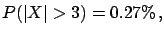 ) only if another generator
  is taken into
account. If this is the case, the probability depends
on the parameters of the generators, the observed value and
on the probability
that the two generators enter the game. For example, if
has
is taken into
account. If this is the case, the probability depends
on the parameters of the generators, the observed value and
on the probability
that the two generators enter the game. For example, if
has  and ,
it is reasonable to think that
and ,
it is reasonable to think that
 |
(1.13) |
Let us imagine a variation of the example:
The generation is performed according to an algorithm
that chooses or , with a
ratio of probability
10 to 1 in favour of . The conclusions change:
Given the same observed value ,
one would tend to infer that is most probably due
to .
It is
not difficult to be convinced that, even if the value is
a bit closer to the centre of generator (for example 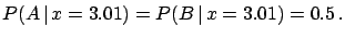 ),
there will still be a tendency to attribute it to .
This
natural way of reasoning is exactly what is meant by `Bayesian',
and will be illustrated in these
notes.1.20. It should be noted that we are
only considering the observed data ( or
), and not other values which could be observed
(
),
there will still be a tendency to attribute it to .
This
natural way of reasoning is exactly what is meant by `Bayesian',
and will be illustrated in these
notes.1.20. It should be noted that we are
only considering the observed data ( or
), and not other values which could be observed
( , for example)
I hope these examples might at least persuade
the reader to take
the question of principles in probability statements seriously.
Anyhow, even if we ignore philosophical aspects,
there are other kinds of more technical inconsistencies
in the way the standard paradigm is used to test hypotheses.
These problems, which deserve extensive discussion,
are effectively
described in an interesting American Scientist
article[10].
At this point I imagine that the reader will have a very
spontaneous and legitimate objection: ``but why does this
scheme of hypothesis tests usually work?''. I will comment
on this question in Section ![[*]](file:/usr/lib/latex2html/icons/crossref.png) , but first we
must introduce the alternative scheme for quantifying uncertainty.
, but first we
must introduce the alternative scheme for quantifying uncertainty.
Next: A probabilistic theory of
Up: Uncertainty in physics and
Previous: Misunderstandings caused by the
Contents
Giulio D'Agostini
2003-05-15