Next: Conventional use of Bayes'
Up: Conditional probability and Bayes'
Previous: Conditional probability
Contents
Bayes' theorem
Let us think of all the possible, mutually exclusive,
hypotheses  which could condition
the event
which could condition
the event  . The problem here is the inverse of the previous one:
what is the probability of under the hypothesis that
has occurred? For example,
``what is the probability that a charged
particle which went in a certain direction and has lost
between 100 and
. The problem here is the inverse of the previous one:
what is the probability of under the hypothesis that
has occurred? For example,
``what is the probability that a charged
particle which went in a certain direction and has lost
between 100 and
 keV
in the detector
is a
keV
in the detector
is a  , a
, a  , a
, a  , or a
  ?" Our event
is ``energy loss between 100 and
keV'',
and
are the four ``particle hypotheses''.
This example sketches the basic problem for
any kind of measurement: having observed an effect,
to assess the probability of each of the causes which
could have produced it. This intellectual
process is called inference, and it will be discussed
in Section
?" Our event
is ``energy loss between 100 and
keV'',
and
are the four ``particle hypotheses''.
This example sketches the basic problem for
any kind of measurement: having observed an effect,
to assess the probability of each of the causes which
could have produced it. This intellectual
process is called inference, and it will be discussed
in Section ![[*]](file:/usr/lib/latex2html/icons/crossref.png) .
.
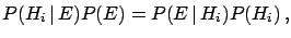
In order to calculate
 let us rewrite the
joint probability
let us rewrite the
joint probability
 , making use of
(-),
in two different ways:
, making use of
(-),
in two different ways:
 |
(3.7) |
obtaining
 |
(3.8) |
or
 |
(3.9) |
Since the hypotheses are mutually exclusive
(i.e.
 ,
,
 ) and exhaustive
(i.e.
) and exhaustive
(i.e.
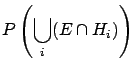
 ),
can be written as
),
can be written as
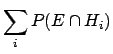
 , the union of the intersections of
with each of the hypotheses . It follows that
, the union of the intersections of
with each of the hypotheses . It follows that
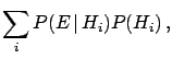
where we have made use of ()
again in the last step.
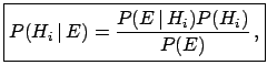
It is then possible to rewrite ()
as
 |
(3.11) |
This is the standard form by which Bayes' theorem
is known. ()
and () are also different ways
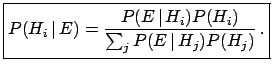
of writing it. As the denominator of
() is nothing but a normalization
factor, such that
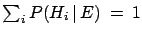 , the formula
() can be
written as
, the formula
() can be
written as
 |
(3.12) |
Factorizing  in (), and explicitly writing
that all the events were already
conditioned by
in (), and explicitly writing
that all the events were already
conditioned by  , we can rewrite the formula
as
, we can rewrite the formula
as
 |
(3.13) |
with
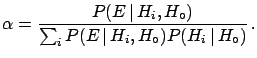 |
(3.14) |
These five ways of rewriting the same formula simply reflect
the importance that we shall give to this simple theorem.
They stress different aspects of the same concept.
- () is the standard way of writing it, although some
prefer ().
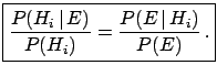
- () indicates that is altered
by the condition with the same ratio with which
 is altered by the condition .
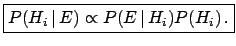
- ()
is the simplest and the most intuitive way to
formulate the theorem: ``the probability of given is
proportional to the initial probability of times
the probability of given ''.
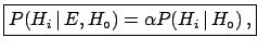
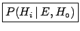
- (-)
show explicitly how
the probability of a certain hypothesis is updated when the
state of information changes:
-

- [also indicated as
 ] is
the initial, or a priori, probability (or simply
``prior'') of , i.e. the probability of this hypothesis
with the state of information available
``before'' the
knowledge that has occurred;
] is
the initial, or a priori, probability (or simply
``prior'') of , i.e. the probability of this hypothesis
with the state of information available
``before'' the
knowledge that has occurred;
-
- [or simply
] is the
final, or ``a posteriori'', probability of
``after''3.7 the new information.
-
- [or simply
 ] is
called likelihood.
] is
called likelihood.
To better understand the terms ``initial'', ``final'' and
``likelihood'', let us formulate the problem in a way closer
to the physicist's mentality, referring to causes and
effects: the causes could be all the physical sources
which may produce a certain observable (the effect). The
likelihoods are -- as the word says -- the
likelihoods that the effect follows from each of the causes.
Using our example of the  measurement again, the
causes are all the possible charged particles which can
pass through the detector; the effect is the amount of observed
ionization;
the likelihoods are the probabilities that each of the particles
give that amount of ionization.
Note that in this example we have fixed all
the other sources of influence: physics process,
HERA running conditions, gas mixture, high voltage,
track direction, etc. This is our .
The problem immediately gets rather complicated (all real cases,
apart from tossing coins and dice, are complicated!).
The real inference would be of the kind
measurement again, the
causes are all the possible charged particles which can
pass through the detector; the effect is the amount of observed
ionization;
the likelihoods are the probabilities that each of the particles
give that amount of ionization.
Note that in this example we have fixed all
the other sources of influence: physics process,
HERA running conditions, gas mixture, high voltage,
track direction, etc. This is our .
The problem immediately gets rather complicated (all real cases,
apart from tossing coins and dice, are complicated!).
The real inference would be of the kind
 |
(3.15) |
For each state (the set of all the possible values
of the influence parameters) one gets a different result
for the final probability3.8.
So, instead of getting a single number
for the final probability we have a distribution of values. This spread
will result in a large uncertainty of
. This is what
every physicist knows: if the calibration constants of the detector
and the physics process are not under control,
the ``systematic errors'' are large and the result is
of poor quality.
Next: Conventional use of Bayes'
Up: Conditional probability and Bayes'
Previous: Conditional probability
Contents
Giulio D'Agostini
2003-05-15