


Next: Covariance matrix of experimental
Up: Bypassing the Bayes' theorem
Previous: Caveat concerning the blind
Contents
Indirect measurements
Conceptually this is a very simple task in the Bayesian framework,
whereas
the frequentistic one requires a lot of gymnastics,
going back and forth from the logical level of true values
to the logical level of estimators. If one accepts that
the true values are just random variables6.6,
then,
calling  a function of other quantities
  ,
each
having a probability density function
,
each
having a probability density function  ,
the probability density function
of
,
the probability density function
of  can be calculated with the
standard formulae
which follow from the rules
probability.
Note that in the approach presented in these notes
uncertainties due to systematic effects
are treated in the same way as indirect measurements.
It is worth repeating that
there is no conceptual
distinction between various components
of the measurement uncertainty.
When approximations are sufficient,
formulae (
can be calculated with the
standard formulae
which follow from the rules
probability.
Note that in the approach presented in these notes
uncertainties due to systematic effects
are treated in the same way as indirect measurements.
It is worth repeating that
there is no conceptual
distinction between various components
of the measurement uncertainty.
When approximations are sufficient,
formulae (![[*]](file:/usr/lib/latex2html/icons/crossref.png) ) and () can be used.
) and () can be used.
Let us take an example for which the linearization does not give
the right result.
- Example:
- The speed of a proton is measured with a time-of-flight
system. Find the
 ,
,  and
and 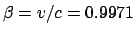 probability intervals
for the energy, knowing that
probability intervals
for the energy, knowing that
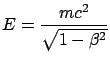 ,
and that distance and time have been measured with a
,
and that distance and time have been measured with a  accuracy.
The relation
is strongly nonlinear. The results given by the approximated method
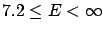
and the correct one are shown in the table below.
| Probability |
Linearization |
Correct result |
| (%) |
 (GeV) (GeV) |
(GeV) |
| 68 |
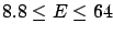 |
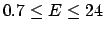 |
| 95 |
 |
 |
| 99 |
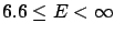 |
 |
Next: Covariance matrix of experimental
Up: Bypassing the Bayes' theorem
Previous: Caveat concerning the blind
Contents
Giulio D'Agostini
2003-05-15