AIDS test

Let us make an example of general interest, that exhibits some of the issues that also arise in forensics.

Imagine an Italian citizen is chosen at random to undergo an AIDS test. Let us assume the analysis used to test for HIV infection is not perfect. In particular, infected people ( HIV) are declared `positive' ( Pos) with 99.9% probability and `negative' ( Neg) with 0.1%; there is, instead, a 0.2% chance a healthy person ( $\overline{\mbox{HIV}}$) is told positive (and 99.8% negative).

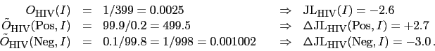
The other information we need is the prevalence of the virus in Italy, from which we evaluate our initial belief that the randomly chosen person is infect. We take 1/400 or 0.25% (roughly 150 thousands in a population of 60 millions).

To summarize, these are the pieces of information relevant to work the exercise:⁵²

$$P( \,\vert\, ,I) = 99.9\%,$$

$$P( \,\vert\, ,I) = 0.1\%,$$

$$P( \,\vert\,\overline{\mbox{HIV}},I) = 0.2\%$$

$$P( \,\vert\,\overline{\mbox{HIV}},I) = 99.8\%$$

$$P( \,\vert\,I) = 0.25\%$$

$$P(\overline{\mbox{HIV}}\,\vert\,I) = 99.75\%,$$

from which we can calculate initial odds, Bayes factors and JL's [we use here the notation $O_{\mbox{{\footnotesize HIV}}}(I)$, instead of our usual $O_{1,2}(I)$ to indicate odds in favor of the hypothesis HIV and against the opposite hypothesis ( $\overline{\mbox{HIV}}$); similarly for JL$_{HIV}$ and $\Delta$JL$_{HIV}$]:

$$\begin{array}{rclcl} O_{\mbox{{\footnotesize HIV}}}(I) &=& 1... ...\mbox{{\footnotesize HIV}}}(\mbox{Neg},I) = -3.0\,. \end{array}$$

A positive result adds a weight of evidence of 2.7 to $-2.6$, yielding the negligible leaning of $+0.1$. Instead a negative result has the negative weight of $-3.0$, shifting the leaning to $-5.6$, definitely on the safe side (see fig. 8).

Figure: AIDS test illustrated with judgement leanings.

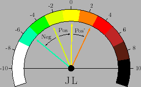
The figure shows also the effect of a second, independent⁵³analysis, having the same performances of the first one and in which the person results again positive. As it clear from the figure, the same conclusion would be reached if only one test was done on a subject for which a doctor could be in serious doubt if he/she had AIDS or not ( JL$\approx 0$).

From this little example we learn that if we want to have a good discrimination power of a test, it should have a $\Delta$JL very large in module. Absolute discrimination can only be achieved if the weight of evidence is infinite, i.e. if either hypothesis is impossible given the observation.