- ...
checkmate.1
- Just writing this note,
I have realized that
the final scene is directed so well
that, not only the way the photographer
loses control and commits his fatal mistake looks very credible,
but also spectators forget he could play valid countermoves,
not depending
on the negative of the pretended destroyed picture
(see footnote 32).
Therefore, rather than chess, the name of
the game is poker, and
Columbo's bluff is able to induce
the murderer to provide a crucial piece of evidence
to finally incriminate him.
.
.
.
.
.
.
.
.
.
.
.
.
.
.
.
.
.
.
.
.
.
.
.
.
.
.
.
.
.
.
- ... trial.2
- This kind of objection,
in defense of what is often nothing but
``the capricious ipse dixit of authority''[5],
from which we should instead ``emancipate''[5],
is quite frequent.
It is raised not only by judges, who tend to claim their job is
"to evaluate evidence not by means of a formula...
but by the joint application of their
individual common sense."[1],
but also by other categories of people
who take important decisions, like
doctors, managers and politicians.
.
.
.
.
.
.
.
.
.
.
.
.
.
.
.
.
.
.
.
.
.
.
.
.
.
.
.
.
.
.
- ...only3
- Beware of methods
that provide `levels of confidence', or something
like that, without using Bayes' theorem! See also
footnote 9 and Appendix H.
.
.
.
.
.
.
.
.
.
.
.
.
.
.
.
.
.
.
.
.
.
.
.
.
.
.
.
.
.
.
- ...
information4
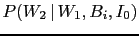
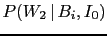
- The background information
 represents all we know about the hypotheses
and the effect considered. Writing in all
expressions could seem a pedantry,
but it isn't.
For example, if we would just write
represents all we know about the hypotheses
and the effect considered. Writing in all
expressions could seem a pedantry,
but it isn't.
For example, if we would just write
 in these formulae, instead of
 ,
one might be tempted to take
this probability equal to one,
``because the observed event is a well established fact',
that has happened and is then certain.
But it is not this certainty
that enters these formulae, but rather the probability `that
fact could happen'
in the light of `everything we knew' about it (`').
,
one might be tempted to take
this probability equal to one,
``because the observed event is a well established fact',
that has happened and is then certain.
But it is not this certainty
that enters these formulae, but rather the probability `that
fact could happen'
in the light of `everything we knew' about it (`').
.
.
.
.
.
.
.
.
.
.
.
.
.
.
.
.
.
.
.
.
.
.
.
.
.
.
.
.
.
.
- ...
theorem.5
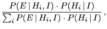
- Bayes' theorem can be often found in the form
valid if we deal with a class of incompatible hypotheses
[i.e.
 and
and
 ].
In fact, in this case
a general rule of probability theory [Eq. (35) in Appendix A]
allows us
to rewrite the denominator of Eq. (3)
as
].
In fact, in this case
a general rule of probability theory [Eq. (35) in Appendix A]
allows us
to rewrite the denominator of Eq. (3)
as
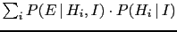 .
In this note, dealing only with two hypotheses,
we prefer to reason in terms of probability ratios,
as shown in Eq. (4).
.
In this note, dealing only with two hypotheses,
we prefer to reason in terms of probability ratios,
as shown in Eq. (4).
.
.
.
.
.
.
.
.
.
.
.
.
.
.
.
.
.
.
.
.
.
.
.
.
.
.
.
.
.
.
- ... effect.6
- Note that,
while in the case of only two hypotheses entering the inferential
game their initial probabilities are related by
 , the probabilities of the effects
 and
and
 have usually nothing to do
with each other.
have usually nothing to do
with each other.
.
.
.
.
.
.
.
.
.
.
.
.
.
.
.
.
.
.
.
.
.
.
.
.
.
.
.
.
.
.
- ...
likely.7
- Those who want to base the inference only
on the probabilities of the observations given the hypotheses,
in order to ``let the data speak themselves'', might be
in good faith, but their noble intention
does dot save them from dire
mistakes [3]. (See also footnotes 9 and
43, as well as Appendix H.)
.
.
.
.
.
.
.
.
.
.
.
.
.
.
.
.
.
.
.
.
.
.
.
.
.
.
.
.
.
.
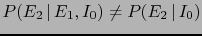
- ... effect.8
- Pieces of evidence
modify, in general,
relative beliefs. When we turn relative beliefs into
absolute ones in a scale ranging from 0 to 1,
we are always making the implicit assumption
that the possible hypotheses are only those
of the class considered.
If other hypotheses are added, the relative beliefs do
not change, while the absolute ones do. This is the reason
why an hypothesis can eventually be falsified, if
 , but an absolute truth, i.e.
 , depends on which class of hypotheses
is considered. Stated in other words,
in the realm of probabilistic inference
falsities can be absolute, but
truths are always relative.
, depends on which class of hypotheses
is considered. Stated in other words,
in the realm of probabilistic inference
falsities can be absolute, but
truths are always relative.
.
.
.
.
.
.
.
.
.
.
.
.
.
.
.
.
.
.
.
.
.
.
.
.
.
.
.
.
.
.
- ... in.9
- You might
be reluctant to adopt this way of reasoning,
objecting
``I am unable to state priors!'', or
``I don't want to be influenced by prior!'', or even
``I don't want to state degrees of beliefs, but only
real probabilities''. No problem, provided you stay
away from probabilistic inference (for example you
can enjoy fishing or hiking - but I hope you are aware of the
large amount of prior beliefs
involved in these activities too!).
Here I can only advice you, provided you are interested in
evaluating probabilities
of `causes' from effects, not to overlook prior information
and not to blindly trust statistical methods and
software packages advertised as prior-free,
unless you don't want to risk to arrive at very bad
conclusions.
For more comments on the question see Ref. [3],
footnote 43 and Appendix H.
.
.
.
.
.
.
.
.
.
.
.
.
.
.
.
.
.
.
.
.
.
.
.
.
.
.
.
.
.
.
- ... one10
-
If
 and
and  are generic, complementary hypotheses
we get, calling
are generic, complementary hypotheses
we get, calling  the Bayes factor of versus
and
the Bayes factor of versus
and  the initial odds to simplify the notation,
the following convenient expressions to evaluate the probability
of :
the initial odds to simplify the notation,
the following convenient expressions to evaluate the probability
of :
.
.
.
.
.
.
.
.
.
.
.
.
.
.
.
.
.
.
.
.
.
.
.
.
.
.
.
.
.
.
- ... now:11
- Note that we
are still using Eq. (4), although we are dealing
now with more complex events and complex hypotheses,
logical AND of simpler ones. Moreover, Eq. (12)
is obtained from Eq. (11) making use of
the formula (2) of joint probability,
that gives
 and an analogous formula for
  .
Note also that, going from
Eq. (12) to Eq. (13),
.
Note also that, going from
Eq. (12) to Eq. (13),
 has been rewritten as
 to emphasize that the probability
of a second white ball,
conditioned by the box composition and the
result of the first extraction,
depends indeed only on the box content
and not on the previous outcome (`extraction after re-introduction').
to emphasize that the probability
of a second white ball,
conditioned by the box composition and the
result of the first extraction,
depends indeed only on the box content
and not on the previous outcome (`extraction after re-introduction').
.
.
.
.
.
.
.
.
.
.
.
.
.
.
.
.
.
.
.
.
.
.
.
.
.
.
.
.
.
.
- ...
i.e.12
- Eq. (17) follows from Eq. (16)
because a Bayes factor can be defined as the ratio
of final odds over the initial odds, depending on the evidence.
Therefore
.
.
.
.
.
.
.
.
.
.
.
.
.
.
.
.
.
.
.
.
.
.
.
.
.
.
.
.
.
.
- ...independent13
- Probabilistic, or `stochastic',
independence of the observations
is related to the
validity of the relation
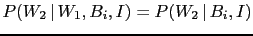 ,
that we have used above to turn
Eq. (12) into Eq. (13) and that can be expressed,
in general terms as
,
that we have used above to turn
Eq. (12) into Eq. (13) and that can be expressed,
in general terms as
i.e., under the condition of a well precise
hypothesis ( ), the probability of the effect
  does not depend on the knowledge of whether
  has occurred or not. Note that, in general,
although and are independent given
(they are said to be conditionally independent),
they might be otherwise dependent, i.e.
has occurred or not. Note that, in general,
although and are independent given
(they are said to be conditionally independent),
they might be otherwise dependent, i.e.
 .
(Going to the
example of the boxes, it is rather easy to grasp,
although I cannot enter in details here,
that, if we do not know the kind of box, the
observation of
.
(Going to the
example of the boxes, it is rather easy to grasp,
although I cannot enter in details here,
that, if we do not know the kind of box, the
observation of  changes our opinion about the box
composition and, as a consequence,
the probability of
changes our opinion about the box
composition and, as a consequence,
the probability of  - see the examples in Appendix J)
.
.
.
.
.
.
.
.
.
.
.
.
.
.
.
.
.
.
.
.
.
.
.
.
.
.
.
.
.
.
- ... quantities.14
- The
idea of transforming a multiplicative updating into
an additive one via the use of logarithms
is quite natural and seems to have
been firstly used in 1878 by Charles Sanders Peirce [6]
and finally introduced in the statistical practice mainly due
to the work of I.J. Good [7].
For more details see the Appendix E.
.
.
.
.
.
.
.
.
.
.
.
.
.
.
.
.
.
.
.
.
.
.
.
.
.
.
.
.
.
.
- ... balance'15
- I have realized only later that
JL sounds a bit like `jail'. That might be not so bad,
if to which
JL
 refers stands for `guilty'.
.
.
.
.
.
.
.
.
.
.
.
.
.
.
.
.
.
.
.
.
.
.
.
.
.
.
.
.
.
.
- ... cases!16
- The
`switch of perspective' from
 to
to
 is done
in a way somewhat automatic if, instead of the probability, we take
the logarithm of the odds, for example our JL (obviously the
base of the logarithm is irrelevant). Since
JL
is done
in a way somewhat automatic if, instead of the probability, we take
the logarithm of the odds, for example our JL (obviously the
base of the logarithm is irrelevant). Since
JL![$ _H(I)=\log_{10}[P(H\,\vert\,I)/P(\overline H\,\vert\,I)]$](img191.png) ,
in the limit
,
in the limit
 we have that
JL
we have that
JL![$ _H(I)\approx \log_{10}[P(H\,\vert\,I)]$](img193.png) , while
the limit
, while
the limit
 it is
JL
it is
JL![$ _H(I)\approx - \log_{10}[P(\overline H\,\vert\,I)]$](img195.png) .
.
.
.
.
.
.
.
.
.
.
.
.
.
.
.
.
.
.
.
.
.
.
.
.
.
.
.
.
.
.
.
- ...
it.17
- This is more or less what happens in measurements.
Take for example the probabilities that appears in the
`monitor' of figure 11: 53.85%
for white and 46.15% for black. This is like to say that
two bodies weigh 53.85g and 46.15g, as resulting
from a measurement with a precise balance (the Bayesian network
tool described in Appendix J applied to the box toy model
is the analogue of the precise balance).
For some purposes two, three and even four significant digits
can be important. But, anyhow, as far as
our perception is concerned, not only the least digits are
absolutely irrelevant but we can hardly distinguish between
54g and 46g.
.
.
.
.
.
.
.
.
.
.
.
.
.
.
.
.
.
.
.
.
.
.
.
.
.
.
.
.
.
.
- ... credible.18
- The following
quotes can be rather enlighting,
especially for those who think they think,
just for educational reasons, `they have to be frequentist':
``Given the state of our knowledge about everything that could
possibly have any bearing on the coming true of a certain event
(thus in dubio: of the sum total of our knowledge),
the numerical probability  of this event is to be a real number
by the indication of which we try in some cases to set up a quantitative
measure of the strength of our conjecture or anticipation, founded
on the said knowledge, that the event comes true.
of this event is to be a real number
by the indication of which we try in some cases to set up a quantitative
measure of the strength of our conjecture or anticipation, founded
on the said knowledge, that the event comes true.
...
Since the knowledge may be different with different persons or with
the same person at different times, they may anticipate the same event
with more or less confidence, and thus different numerical probabilities
may be attached to the same event. ... Thus
whenever we speak loosely of the `probability of an event,'
it is always to be understood: probability with regard to a certain
given state of knowledge.'' [11]
.
.
.
.
.
.
.
.
.
.
.
.
.
.
.
.
.
.
.
.
.
.
.
.
.
.
.
.
.
.
- ... precision.19
- Those
who are not familiar with this
approach have understandable
initial difficulties and risk to be at lost.
A formula, they might argue,
can be of practical use only if we can replace
the symbols by numbers, and in pure mathematics a number
is a well defined
object, being, for example, 49.999999 different from
50.
Therefore, they might conclude that, being unable to
choose the number, the above formulae, that
seem to work nicely in die/coin/ball games, are
useless in other domains of applications (the most
interesting of all, as it was clear already centuries ago
to Leibniz and Hume).
But in the realm of uncertainty things go quite differently,
as everybody understands, apart from hypothetical
Pythagorean monks living in a ivory monastery.
For practical purposes not only 49.999999% is `identical'
to 50%, but also 49% and 51%
give to our mind essentially the same
expectations of what it could occur.
In practice we are interested to
understand if somebody else's degrees of belief
are low, very low, high, very very high, ad so on.
And the same is what other people expect from us.
.
.
.
.
.
.
.
.
.
.
.
.
.
.
.
.
.
.
.
.
.
.
.
.
.
.
.
.
.
.
- ...
respectively.20
-
That is, the final probability of would range between 99.90%
and 99.999% in the first case,
between 0.001% and 0.1% in the second one,
making us `practically sure' of either hypothesis
in the two cases.
.
.
.
.
.
.
.
.
.
.
.
.
.
.
.
.
.
.
.
.
.
.
.
.
.
.
.
.
.
.
- ...frequentism.21
- Sometimes
frequency is even confused with `proportion'
when it is said, for example, that the probability
is evaluated thinking how many persons in a given
population would behave in a given way, or have a
well defined character.
.
.
.
.
.
.
.
.
.
.
.
.
.
.
.
.
.
.
.
.
.
.
.
.
.
.
.
.
.
.
- ...
average.22
- The reason behind it is rather easy
to grasp. When we have uncertain beliefs
it is like if our mind oscillates among possible
values, without being able to choose an exact value.
Exactly as it happens when we try to guess, just by eye,
the length of a stick, the weight of an object or a
temperature in a room: extreme values are
promptly rejected, and our judgement oscillates in an interval,
whose width depends on our estimation ability, based on
previous experience.
Our guess will be somehow the center of the interval.
The following minimalist example helps to understand
the rule of combination of uncertain evaluations.
Imagine that the (not better
defined) quantities
 and
and  might each
have, in our opinion,
the values 1, 2 or 3,
among which we are unable to choose.
If we now think of a
might each
have, in our opinion,
the values 1, 2 or 3,
among which we are unable to choose.
If we now think of a  , its value can then range between
2 and 6. But, if our mind oscillates uniformly and independently
over the three possibilities of and , the oscillation
over the values of
, its value can then range between
2 and 6. But, if our mind oscillates uniformly and independently
over the three possibilities of and , the oscillation
over the values of  is not uniform. The reason is that
  can is only related to
  and
and  . Instead, we think at
 if we think at and
  , or at
  and .
Playing with a cross table of possibilities, it is rather
easy to prove that
and .
Playing with a cross table of possibilities, it is rather
easy to prove that  gets
a weight three times larger than that of .
We can add a third quantity
gets
a weight three times larger than that of .
We can add a third quantity  , similar to and ,
and continue the exercise, understanding then the essence of
what is called in probability theory central limit theorem,
which then applies also to the weight of our JL's.
[Solution and comment: if
, similar to and ,
and continue the exercise, understanding then the essence of
what is called in probability theory central limit theorem,
which then applies also to the weight of our JL's.
[Solution and comment: if  , the weights of the 7 possibilities, from 3 to 9
are in the following proportions: 1:3:6:7:6:3:1. Note that, contrary
to , the weights do not go linearly up and down, but there is
a non-linear concentration at the center. When many variables of this
kind are combined together, then the distribution
of weights exhibits the well known bell shape of the Gaussian distribution.
The widths of the red arrows in figure 4
tail off from the central one according to a Gaussian function.]
, the weights of the 7 possibilities, from 3 to 9
are in the following proportions: 1:3:6:7:6:3:1. Note that, contrary
to , the weights do not go linearly up and down, but there is
a non-linear concentration at the center. When many variables of this
kind are combined together, then the distribution
of weights exhibits the well known bell shape of the Gaussian distribution.
The widths of the red arrows in figure 4
tail off from the central one according to a Gaussian function.]
.
.
.
.
.
.
.
.
.
.
.
.
.
.
.
.
.
.
.
.
.
.
.
.
.
.
.
.
.
.
- ...
uniformly23
- It easy to understand that if the
judgement would be uniform in the odds, ranging then from
1 to 10, the conclusion could be different. Here it
is assumed that the `intensity of belief'[6]
is proportional to the logarithm of the odds, as
extensively discussed in Appendix E.
.
.
.
.
.
.
.
.
.
.
.
.
.
.
.
.
.
.
.
.
.
.
.
.
.
.
.
.
.
.
- ... leanings24
- Using the language of footnote
22, this is the range in which
the minds oscillate in 95% of the times when thinking of
 JL
JL .
.
.
.
.
.
.
.
.
.
.
.
.
.
.
.
.
.
.
.
.
.
.
.
.
.
.
.
.
.
.
.
- ... enough.25
- I wish
judges state Bayes factors
of each piece of evidence, as vaguely as
they like
(much better than telling nothing! - Bruno
de Finetti was used to say that ``it is better
to build on sand that on void''),
instead of saying that somebody is
guilty ``behind any reasonable doubt'' -
and I am really curious to check to what
degree of belief that
level of doubt corresponds!
.
.
.
.
.
.
.
.
.
.
.
.
.
.
.
.
.
.
.
.
.
.
.
.
.
.
.
.
.
.
- ...
valid.26
- What to do in this case?
As it easy to imagine, when the structure of dependencies
among evidences is complex, things might become
quite complicated. Anyway, if one is able to isolate
two o more pieces of evidence that are
correlated with themselves
(let they be and ), then, one can consider
the joint event
 as the effective evidence to be used.
In the extreme case in which implies logically
(think at the events `even' and '2' rolling a die),
then
as the effective evidence to be used.
In the extreme case in which implies logically
(think at the events `even' and '2' rolling a die),
then
 , from which it follows that
 : the second evidence
is therefore simply superfluous.
: the second evidence
is therefore simply superfluous.
.
.
.
.
.
.
.
.
.
.
.
.
.
.
.
.
.
.
.
.
.
.
.
.
.
.
.
.
.
.
- ...
possibility.27
- When we are called to make
critical decisions
even very remote hypotheses,
although with very low probability,
should be present to our minds
- that is
Dennis Lindley's
Cromwell's rule [18].
[The very recent news from New York
offer material for reflection [19].]
.
.
.
.
.
.
.
.
.
.
.
.
.
.
.
.
.
.
.
.
.
.
.
.
.
.
.
.
.
.
- ... doubts.28
- Again, my impression comes
from media, literature and fiction, but I cannot see how
`casual judges' can be better than professional ones
to evaluate all elements of a complex trial, or how to
distinguish sound arguments from pure rhetoric of the
lawyers. This is particularly true when the `network of evidences'
is so intricate that even well trained human minds
might have difficulties, and artificial intelligence
tools would be more appropriated (see Appendices C and J).
.
.
.
.
.
.
.
.
.
.
.
.
.
.
.
.
.
.
.
.
.
.
.
.
.
.
.
.
.
.
- ... beliefs29
- See Appendices C and J.
.
.
.
.
.
.
.
.
.
.
.
.
.
.
.
.
.
.
.
.
.
.
.
.
.
.
.
.
.
.
- ... mind30
- Obviously,
saying Columbo has a network of beliefs in his head,
I don't mean he is thinking at these mathematical tools.
On the other way around, these tools try to model
the way we reason, with the advantage they
can better handle complex
situations (see Appendices C and J).
.
.
.
.
.
.
.
.
.
.
.
.
.
.
.
.
.
.
.
.
.
.
.
.
.
.
.
.
.
.
- ...
suit.31
- There is, for example, the interesting
case of the clochard who
was on the scene of the crime and, although still drunk,
tells, among other verifiable things, to have heard two gun shots
with a remarkable
time gap in between, something in absolute contradiction
with Galesco reconstruction of the facts, in which he
states to have killed Alvin Deschler,
that he pretends to be the kidnapper
and murderer of his wife, for self-defense,
thus shooting practically simultaneously with him.
Unfortunately, days after,
when the clochard is interviewed by Columbo, he says,
apparently honestly,
to remember nothing of what happened the day of the crime,
because
he was completely drunk. He confesses he
doesn't even remember what he
declared to the police immediately after.
Therefore he could never be able to testify
in a court. However, it is difficult an investigator
would remove such a
piece of evidence from his mind, a piece of evidence
that fits well with the alternative hypothesis
that starts to account better for many other major and minor
details.
He knows he cannot present it to the court,
but it pushes him to go further, looking for more
`presentable' pieces of evidence, and possibly
for conclusive
proofs.
.
.
.
.
.
.
.
.
.
.
.
.
.
.
.
.
.
.
.
.
.
.
.
.
.
.
.
.
.
.
- ... reversed.32
- In reality
he has several ways out, not depending on that negative
(this could be a weak point of the story, but it is
plausible, and the dramatic force of the action induces also
TV watchers to neglect this particular, as my friends and I have
experienced):
- He knew
Columbo owns a second picture, discarded by the killer
because of minor defects
and left on the crime scene.
(That was one of the several hints against Galesco, because only
a maniac photographer - and certainly not
Alvin Deschler - would care of
the artistic quality of a picture shot just to prove
a person was in his hands - think at the very poor quality
pictures from real kidnappers and terrorists).
- As an expert photographer, he had to think that
the asymmetries in the picture would save him.
In particular
- The picture shows an asymmetric disposition of the
furniture. Obviously he cannot tell which one is the correct
one, but he could simply say that he was so sure it was
2:00 PM that, for example, the dresser had to be right of
fireplace and not on its left. He could simply require to check it.
- Finally, his wife wore a white rosette on her left.
This detail would allow him to claim with certainty
that the picture has been reversed (he knew how his wife
was dressed, something that could be easily verified by the police,
and, moreover, rosettes hang regularly left).
.
.
.
.
.
.
.
.
.
.
.
.
.
.
.
.
.
.
.
.
.
.
.
.
.
.
.
.
.
.
- ... cameras.33
- Nobody
mentioned the camera was
in those shelfs or even in that room!
(And TV watchers didn't get the
information that
Galesco knew that the camera was found by the police - but
this could just be a minor detail.)
Moreover, only the killer and few policemen
knew that the negative was left inside it by the
murderer, a particular that is no obvious at all. As it was
very improbable the killer used such an old-fashioned of
camera.
Note in fact that the camera
was considered a quite old one
already at the time the episode was set
and it was bought in a second hand shop.
In fact I remember being wondering
about that writer's choice,
until the very end:
it was done on the purpose, so that nobody but the
killer could think it was used to snap Mrs Galesco.
Clever!
.
.
.
.
.
.
.
.
.
.
.
.
.
.
.
.
.
.
.
.
.
.
.
.
.
.
.
.
.
.
- ... probable'34
- Note
that it is not required that one of the
hypotheses should give with probability one,
as it occurred instead of the toy example of section
2. (See also Appendix G.)
.
.
.
.
.
.
.
.
.
.
.
.
.
.
.
.
.
.
.
.
.
.
.
.
.
.
.
.
.
.
- ... them.35
- A quote
by David Hume is in order (the subdivision
in paragraphs is mine):
All reasonings concerning matter of fact seem to be founded
on the relation of Cause and Effect.
By means of that relation alone we can go beyond the evidence
of our memory and senses.
If you were to ask a man, why he believes any matter of fact,
which is absent; for instance, that his friend is in the country,
or in France; he would give you a reason;
and this reason would be some other fact;
as a letter received from him, or the knowledge
of his former resolutions and promises.
A man finding a watch or any other machine in a desert island,
would conclude that there had once been men in that island.
All our reasonings concerning fact are of the same nature.
And here it is constantly supposed that there is a connexion
between the present fact and that which is inferred from it.
Were there nothing to bind them together, the inference
would be entirely precarious.
The hearing of an articulate voice and rational discourse
in the dark assures us of the presence of some person:
Why? because these are the effects of the human make
and fabric, and closely connected with it.
If we anatomize all the other reasonings of this nature,
we shall find that they are founded on the relation
of cause and effect, and that this relation is either
near or remote, direct or collateral.''
[17]
I would like to observe that too often we tend to take for
granted `a fact', forgetting that we didn't really observed
it, but we are relying on a chain of testimonies and assumptions
that lead to it. But some
of them might fail (see footnote 27 and Appendix I).
.
.
.
.
.
.
.
.
.
.
.
.
.
.
.
.
.
.
.
.
.
.
.
.
.
.
.
.
.
.
- ...
flavors36
- Already in 1950 I.J. Good listed in Ref. [7]
9 `theories of probability', some of which could be
called `Bayesian' and among which de Finetti's approach,
just to make an example, does not appear.
.
.
.
.
.
.
.
.
.
.
.
.
.
.
.
.
.
.
.
.
.
.
.
.
.
.
.
.
.
.
- ... occurs.37
- It is
very interesting to observe how people are differently
surprised, in the sense of their emotional reaction,
depending on the occurrence of events that they considered
more or less probable. Therefore, contrary to I.J. Good
- I have been a quite surprised about this - according to
whom
``to say that one degree of belief is more intense than another
one is not intended to mean that there is more emotion attached
to it''[7], I am definitively closer to the position
of Hume:
Nothing is more free than the imagination of man; and though it
cannot exceed that original stock of ideas furnished by the internal and
external senses, it has unlimited power of mixing, compounding,
separating, and dividing these ideas, in all the varieties of fiction
and vision. It can feign a train of events, with all the appearance of
reality, ascribe to them a particular time and place, conceive them as
existent, and paint them out to itself with every circumstance, that
belongs to any historical fact, which it believes with the greatest
certainty. Wherein, therefore, consists the difference between such a
fiction and belief? It lies not merely in any peculiar idea, which is
annexed to such a conception as commands our assent, and which is
wanting to every known fiction. For as the mind has authority over all
its ideas, it could voluntarily annex this particular idea to any
fiction, and consequently be able to believe whatever it pleases;
contrary to what we find by daily experience. We can, in our conception,
join the head of a man to the body of a horse; but it is not in our
power to believe that such an animal has ever really existed.
It follows, therefore, that the difference between fiction and
belief lies in some sentiment or feeling, which is annexed to the
latter, not to the former.
[17]
.
.
.
.
.
.
.
.
.
.
.
.
.
.
.
.
.
.
.
.
.
.
.
.
.
.
.
.
.
.
- ... case,38
- To state it in an explicit way,
I admit, contrary to others, that probability values
can be themselves uncertain, as discussed in footnote
22. I understand that probabilistic
statements about probability values might seem strange concepts
(and this is the reason why I tried to avoid them in footnote
22), but I see nothing unnatural in
statements of the kind ``I am 50% confidence
that the expert will provide a value of probability in the
range between 0.4 and 0.6'', as I would be ready to place
a 1:1 bet on the event that the quoted probability value will be
in that interval or outside it.
.
.
.
.
.
.
.
.
.
.
.
.
.
.
.
.
.
.
.
.
.
.
.
.
.
.
.
.
.
.
- ... zero).39
- I have just learned from Ref. [7] of the following
Sherlock Holmes' principle: ``If a hypothesis
is initially very improbable but is the only one that
explains the facts,then it must be accepted''. However,
a few lines after, Good warns us that ``if the
only hypothesis that seems to explains the facts has very
small initial odds, then this is itself evidence that
some alternative hypotheses has been overlooked''...
.
.
.
.
.
.
.
.
.
.
.
.
.
.
.
.
.
.
.
.
.
.
.
.
.
.
.
.
.
.
- ... probability,40
- Sometimes one hears of axiomatic approach
(or even axiomatic interpretation - an expression
that in my opinion has very little sense)
of probability, also known as axiomatic Kolmogorov approach.
In this approach `probabilities' are just real `numbers' in the range
![$ [0,1]$](img268.png) that satisfy the axioms,
with no interest on their meaning,
i.e. how they are perceived by the human mind.
This kind of approach
might be perfect for a pure mathematician, only interested to
develop all mathematical consequences of the axioms.
However it is not suited for applications, because, before we can use
the `numbers' resulting from such a probability theory,
we have to understand what they mean. For this reason one
might also hear
that ``probabilities are real numbers which obey the axioms
and that we need to `interpret' them'', an expression I deeply dislike.
I like much more the other way around: probability is probability
(how much we believe something) and probability
values can be proved to obey the four basic rules
listed above, which can then considered by a pure mathematician
the `axioms' from which a theory of probability can be built.
that satisfy the axioms,
with no interest on their meaning,
i.e. how they are perceived by the human mind.
This kind of approach
might be perfect for a pure mathematician, only interested to
develop all mathematical consequences of the axioms.
However it is not suited for applications, because, before we can use
the `numbers' resulting from such a probability theory,
we have to understand what they mean. For this reason one
might also hear
that ``probabilities are real numbers which obey the axioms
and that we need to `interpret' them'', an expression I deeply dislike.
I like much more the other way around: probability is probability
(how much we believe something) and probability
values can be proved to obey the four basic rules
listed above, which can then considered by a pure mathematician
the `axioms' from which a theory of probability can be built.
.
.
.
.
.
.
.
.
.
.
.
.
.
.
.
.
.
.
.
.
.
.
.
.
.
.
.
.
.
.
- ... nature.41
- I find that
the following old joke conveys well the message.
A philosopher, a physicist and a mathematician travel by train through
Scotland.
The train is going slowly and they see a cow walking along a country road
parallel to the railway. The philosopher look at the others,
then very seriously states ``In Scotland cows are black''.
The physicist replies that we cannot make such a generalization
from a single individual. We are only authorized to state, he maintains,
that ``In Scotland there is at least one black cow''.
The mathematician looks well at cow,
thinks a while, and then, he said,
``I am afraid you are both incorrect. The most
we can say is that in Scotland at least one cow has a black side''.
.
.
.
.
.
.
.
.
.
.
.
.
.
.
.
.
.
.
.
.
.
.
.
.
.
.
.
.
.
.
- ... frequency.42
- The
following de Finetti's quote is in order.
``For those who seek to connect the notion of probability
with that of frequency,
results which relate probability and frequency
in some way (and especially those
results like the `law of large numbers') play a pivotal rôle,
providing support for the approach and for the identification
of the concepts. Logically speaking, however, one cannot escape
from the dilemma posed by the fact that the same thing cannot both
be assumed first as a definition and then proved as a theorem; nor
can one avoid the contradiction that arises from a definition which
would assume as certain something that the theorem only states
to be very probable.'' [10]
.
.
.
.
.
.
.
.
.
.
.
.
.
.
.
.
.
.
.
.
.
.
.
.
.
.
.
.
.
.
- ... Bayesians'43
- This expression
refers the robot of E.T. Jaynes' [9] and followers,
according to which probabilities should not be subjective.
Nevertheless, contrary to frequentists, they allow the possibility
of `probability inversions' via Bayes' theorem,
but they have difficulties with priors, that, according to them,
shouldn't be subjective. Their solution is that
the evaluation of priors should be then
delegated to some `principles'
(e.g. Maximum Entropy or Jeffrey priors).
But it is a matter of fact that
unnecessary principles (that can be, anyway, used
as convenient rules in particular, well understood situations)
are easily misused (see e.g. comments on maximum
likelihood principle in the Appendix H
- several years ago, remarking this attitude by several
Bayesian fellows, I wrote a note on
Jeffreys priors versus experienced physicist priors;
arguments against objective Bayesian theory,
whose main contents went lately into Ref. [26]),
the approach
becomes dogmatic and uncritical use of some methods
might easily lead to absurd conclusions.
For comments on
anti-subjective criticisms
(mainly those expressed in chapter 12
of Ref. [9]), see section 5 of Ref. [22].
As an example of a bizarre result, although considered
by many Jaynes' followers as one of the jewels of their
teacher's thought, let me mention the famous die problem.
``A die has been tossed a very large number
 of times, and we
are told that the average number of spots up per
toss was not 3.5, as we might expect from an honest die,
but 4.5. Translate this information into a probability
assignment
of times, and we
are told that the average number of spots up per
toss was not 3.5, as we might expect from an honest die,
but 4.5. Translate this information into a probability
assignment
 , for the
  -th face
to come up on the next toss.''[23]
The celebrated Maximum Entropy solution is that the
probabilities for the six faces are,
in increasing order, 5.4%, 7.9%, 11.4%, 18.5%, 24.0%
and 34.8%. I have several times raised my perplexities
about the solution, but the reaction of Jaynes' followers
was, let's say, exaggerated.
Recently this result has been questioned
by the somewhat quibbling Ref. [24]
(one has to recognize that
the original formulation of the problem had anyhow the assumption
that the die was tossed a large number of times),
which, however, also misses
the crucial point: numbers on a die faces are just
labels, having no intrinsic order,
as instead it would be the case of
the indications on a measuring device.
I find absurd
making this kind of inferences without even giving a look
at a real die! (Any reasonable person, used to try to observe
and understand nature,
would first observe careful a die and try to guess
how it could have been loaded to favor the faces having
larger number of spots.)
-th face
to come up on the next toss.''[23]
The celebrated Maximum Entropy solution is that the
probabilities for the six faces are,
in increasing order, 5.4%, 7.9%, 11.4%, 18.5%, 24.0%
and 34.8%. I have several times raised my perplexities
about the solution, but the reaction of Jaynes' followers
was, let's say, exaggerated.
Recently this result has been questioned
by the somewhat quibbling Ref. [24]
(one has to recognize that
the original formulation of the problem had anyhow the assumption
that the die was tossed a large number of times),
which, however, also misses
the crucial point: numbers on a die faces are just
labels, having no intrinsic order,
as instead it would be the case of
the indications on a measuring device.
I find absurd
making this kind of inferences without even giving a look
at a real die! (Any reasonable person, used to try to observe
and understand nature,
would first observe careful a die and try to guess
how it could have been loaded to favor the faces having
larger number of spots.)
.
.
.
.
.
.
.
.
.
.
.
.
.
.
.
.
.
.
.
.
.
.
.
.
.
.
.
.
.
.
- ...
prize.44
- Reading the draft of this paper, my colleague
Enrico Franco has remarked
that in the way the box problems (or the Monthy Hall) are
presented there are additional pieces of information which are usually
neglected, as I also did in Ref. [3]
(`then' was not underlined in the original):
(1) In the first case, imagine two contestants, each of whom
chooses one box at random. Contestant  opens his chosen
box and finds it does not contain the prize. Then the
presenter offers player
opens his chosen
box and finds it does not contain the prize. Then the
presenter offers player  the opportunity to exchange his
box, still un-opened, with the third box. ...
the opportunity to exchange his
box, still un-opened, with the third box. ...
(2) In the second case there is only one contestant, .
After he has chosen one box the presenter tells him that,
although the boxes are identical, he knows which one contains the prize.
Then he says that, out of the two remaining boxes,
he will open one that does not
contain the prize.... [3]
It makes quite some difference if the conductor announces
he will
propose the exchange
before the boxe(s) is/are initially
taken by the contestant(s) that, or if he does it later, as I usually
formulate the problems. In the latter case, in fact, contestant
can have a legitimate doubt concerning the malicious intention of the
conductor, who might want to induce him to lose.
Mathematics oriented guys
would argue then that the problem does have a solution.
But the question is that in real life
one has to act,
and one has to finally make his decision, based on the best
knowledge of the game and of the conductor,
in a finite amount of time.
.
.
.
.
.
.
.
.
.
.
.
.
.
.
.
.
.
.
.
.
.
.
.
.
.
.
.
.
.
.
- ... (isomorph45
- This is true
only neglecting the complication taken into account
in the previous footnote. Indeed, in one case
the `exchange game' is initiated by the conductor,
while in the second by the prisoner,
therefore Enrico Franco's comment does not apply to
the three prisoner problem.
.
.
.
.
.
.
.
.
.
.
.
.
.
.
.
.
.
.
.
.
.
.
.
.
.
.
.
.
.
.
- ... infinity;46
- In this respect,
belief becomes similar
to other human sentiments, for which in normal speech we use a scale that
goes to infinity - think at expressions like `infinite love',
`infinite hate', and so on
(see also footnote 37).
.
.
.
.
.
.
.
.
.
.
.
.
.
.
.
.
.
.
.
.
.
.
.
.
.
.
.
.
.
.
- ...Good.47
- Peirce article is a mix of
interesting intuitions and confused arguments, as in the
``bag of beans'' example of pages 709-710
(he does not understand the difference
between the observation of 20 black beans
and that of 1010 black and 990 white for the
evaluation of the probability that another bean extracted
from the same bag is white or black, arriving thus
to a kind of paradox - from Bayes' rule it is clear
that weights of evidence sum up to form the intensity
of belief on two bag compositions, not
on the outcomes from the boxes [27]). Of a different class is
Good's book, one of the best on probabilistic reasoning
I have met so far, perhaps because I feel myself
often in tune with Good thinking (including the passion
for footnotes and internal cross references shown in Ref. [7]).
.
.
.
.
.
.
.
.
.
.
.
.
.
.
.
.
.
.
.
.
.
.
.
.
.
.
.
.
.
.
- ... odds.48
- But Goods mentions that ``In 1936 Jeffreys
had already appreciated the importance of the logarithm
of the [Bayes] factor and had suggested for it the name
`support'.'' [7]
.
.
.
.
.
.
.
.
.
.
.
.
.
.
.
.
.
.
.
.
.
.
.
.
.
.
.
.
.
.
- ... notation49
- ``In acoustic and electrical engineering
the bel is the logarithm to base 10 of the ratio of
two intensities of sound. Similarly, if
 is the [Bayes] factor
in favor of a hypothesis has gained
is the [Bayes] factor
in favor of a hypothesis has gained
 bels, or
 db.'' [7]
[Good uses the name `factor' for what we call Bayes factor,
``the factor by which the initial odds of
db.'' [7]
[Good uses the name `factor' for what we call Bayes factor,
``the factor by which the initial odds of  must be multiplied in order to obtain the final odds.
Dr. A.M. Turing suggested in a conversation in 1940
that the word `factor' should be regarded as the technical
term in this connexion, and that it could be more fully
described as the factor in favor of the hypothesis
in virtue of the result of the experiment.'' [7]]
must be multiplied in order to obtain the final odds.
Dr. A.M. Turing suggested in a conversation in 1940
that the word `factor' should be regarded as the technical
term in this connexion, and that it could be more fully
described as the factor in favor of the hypothesis
in virtue of the result of the experiment.'' [7]]
.
.
.
.
.
.
.
.
.
.
.
.
.
.
.
.
.
.
.
.
.
.
.
.
.
.
.
.
.
.
- ...
meanings.50
- Many controversies in
probability and statistics arise because there
is no agreement on the meaning of the words
(including `probability' and `statistics'),
or because some refuse to accept this
fact. For example, I am perfectly aware
that many people, especially my friends physicists,
tend to to assign to the word `probability' the meaning
of a kind of propension `nature' has to behave
more in a particular way than in other way,
although in many other cases - and more often! -
they also mean by the same word
how much they believe
something (see e.g. chapters 1 and 10 of Ref. [3]).
For example, one might like to think that kind
 boxes of section 2 have a 100%
propensity to produce white balls and 0
to produce black balls, while type
have 7.7% propension to produce white
and 92.3% to produce black. Therefore, if one
knows the box composition and
is only interested to the outcome of the extraction, then
probability and propensity coincide in value. But if the composition
is unknown this is no longer true, as we shall see
in Appendix J. [By the way, all interesting
questions we shall see in Appendix J have no meaning (and no
clean answers) for ideologizied guy who refuse to accept
that probability primarily means how much we believe something.
(See also comments in Appendix H.)]
boxes of section 2 have a 100%
propensity to produce white balls and 0
to produce black balls, while type
have 7.7% propension to produce white
and 92.3% to produce black. Therefore, if one
knows the box composition and
is only interested to the outcome of the extraction, then
probability and propensity coincide in value. But if the composition
is unknown this is no longer true, as we shall see
in Appendix J. [By the way, all interesting
questions we shall see in Appendix J have no meaning (and no
clean answers) for ideologizied guy who refuse to accept
that probability primarily means how much we believe something.
(See also comments in Appendix H.)]
.
.
.
.
.
.
.
.
.
.
.
.
.
.
.
.
.
.
.
.
.
.
.
.
.
.
.
.
.
.
- ... Good51
-
 .
.
.
.
.
.
.
.
.
.
.
.
.
.
.
.
.
.
.
.
.
.
.
.
.
.
.
.
.
.
.
.
- ... exercise:52
- The performance of the test
are of pure fantasy, while the prevalence is somehow
realistic, although not pretended to be the real one.
But it will be clear that the result is rather insensitive
on the precise figures.
.
.
.
.
.
.
.
.
.
.
.
.
.
.
.
.
.
.
.
.
.
.
.
.
.
.
.
.
.
.
- ...independent53
- Note that `independent' does not mean
the analysis has simply been done by somebody else,
possibly in a different laboratory, but also that the principle
of measurement is independent.
.
.
.
.
.
.
.
.
.
.
.
.
.
.
.
.
.
.
.
.
.
.
.
.
.
.
.
.
.
.
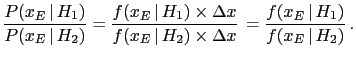
- ... are54
- The curves
 in figure 9
represent probability density functions (`pdf'),
i.e. they give the probability per unit , i.e.
in figure 9
represent probability density functions (`pdf'),
i.e. they give the probability per unit , i.e.
![$ P([x-\Delta x/2,x+\Delta x/2])/\Delta x$](img349.png) ,
for small
,
for small  (remember that `densities' are always local).
Rounding to the 7-th digit means that the number before
rounding was in the interval of
(remember that `densities' are always local).
Rounding to the 7-th digit means that the number before
rounding was in the interval of
 centered
  . It follows that the probability a generator
would produce that number can be calculated as
. It follows that the probability a generator
would produce that number can be calculated as
 . Indeed, we can see
that in the calculation of Bayes factors the width simplifies
and what really matter is the ratio of the two pdf's, i.e.
. Indeed, we can see
that in the calculation of Bayes factors the width simplifies
and what really matter is the ratio of the two pdf's, i.e.
The Bayes factor is therefore the ratio
of the ordinates of the curves in figure 9
for the same . Note that
 can be small at will,
but, nevertheless, hypothesis can receive
a very high weight of evidence from
if
can be small at will,
but, nevertheless, hypothesis can receive
a very high weight of evidence from
if
 .
.
.
.
.
.
.
.
.
.
.
.
.
.
.
.
.
.
.
.
.
.
.
.
.
.
.
.
.
.
.
.
- ...
small''.55
- Sometimes this might be
qualitatively correct, because it easy to imagine
there could be
an alternative hypothesis
 such that:
-
 , such that
the Bayes factor is strongly in favor of ;
, such that
the Bayes factor is strongly in favor of ;
-
 , that is
is roughly as credible as .
, that is
is roughly as credible as .
(For details see section 10.8 of Ref.[3].)
.
.
.
.
.
.
.
.
.
.
.
.
.
.
.
.
.
.
.
.
.
.
.
.
.
.
.
.
.
.
- ....56
- We can evaluate the prevision
(`expected value')
of the variation of leaning at each random extraction for each hypotheses,
calculated as the average value of
JL
 .
We can also evaluate the uncertainty of prevision,
quantified by the standard deviation. We get for the two hypotheses
.
We can also evaluate the uncertainty of prevision,
quantified by the standard deviation. We get for the two hypotheses
where also the relative uncertainty  has been reported,
defined as the uncertainty divided by the absolute
value of the prevision.
The fact that the uncertainties are relatively
large tells clearly
that we do not expect that
a single extraction will be sufficient to convince us of
either model.
But this does not mean we cannot take the decision
because the number of extraction has been too small.
If a very large fluctuation provides a JL of
has been reported,
defined as the uncertainty divided by the absolute
value of the prevision.
The fact that the uncertainties are relatively
large tells clearly
that we do not expect that
a single extraction will be sufficient to convince us of
either model.
But this does not mean we cannot take the decision
because the number of extraction has been too small.
If a very large fluctuation provides a JL of  (the table in this section shows that this is not very rare),
we have already got a very strong evidence in favor of .
Repeating what has been told several time, what matters
is the cumulated judgement leaning. It is irrelevant
if a JL of comes from ten individual pieces of evidence,
only from a single one, or partially from evidence
and partially from prior judgement.
(the table in this section shows that this is not very rare),
we have already got a very strong evidence in favor of .
Repeating what has been told several time, what matters
is the cumulated judgement leaning. It is irrelevant
if a JL of comes from ten individual pieces of evidence,
only from a single one, or partially from evidence
and partially from prior judgement.
When we plan to make extractions from a generator,
probability theory allows
us to calculate expected value and uncertainty of
JL :
:
In particular, for  we get
JL
we get
JL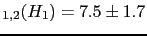 (
( )
and
JL
)
and
JL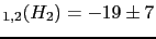 (
( ), that
explain the gross feature of the bands in
figure 10.
), that
explain the gross feature of the bands in
figure 10.
.
.
.
.
.
.
.
.
.
.
.
.
.
.
.
.
.
.
.
.
.
.
.
.
.
.
.
.
.
.
- ...
`irregular'57
- I find the issue of
`statistical regularities' to be often misunderstood.
For example, the trajectories in figure 10
that do not follow the general trend are not exceptions,
being generated by the same rules that produces all of them.
.
.
.
.
.
.
.
.
.
.
.
.
.
.
.
.
.
.
.
.
.
.
.
.
.
.
.
.
.
.
- ...
probable''58
- See e.g.
http://www.thefreedictionary.com/likelihood.
.
.
.
.
.
.
.
.
.
.
.
.
.
.
.
.
.
.
.
.
.
.
.
.
.
.
.
.
.
.
- ...
`likelihood'.59
- Note added: I have just learned,
while making the short
research on the use of the logarithmic updating of the odds
presented in Appendix E, that ``the term [likelihood]
was introduced by R. A. Fisher with the object of
avoiding the use of Bayes' theorem'' [7].
.
.
.
.
.
.
.
.
.
.
.
.
.
.
.
.
.
.
.
.
.
.
.
.
.
.
.
.
.
.
- ....60
-
As further example, you might look at
http://en.wikipedia.org/wiki/Likelihood_principle, where
it is stated (January 28, 2010, 15:40)
that a likelihood
``gives a measure of how `likely' any particular value of
 is''
(note the quote mark of `likely', as in the example of footnote
61).
But, fortunately we
find in http://en.wikipedia.org/wiki/Likelihood_function that
``This is not the same as the probability that those parameters
are the right ones, given the observed sample.
Attempting to interpret the likelihood of a hypothesis
given observed evidence as the probability of the hypothesis
is a common error, with potentially disastrous real-world
consequences in medicine, engineering or jurisprudence.
See prosecutor's fallacy[*] for an example of this.''
([*] see
http://en.wikipedia.org/wiki/Prosecutor%27s_fallacy.)
is''
(note the quote mark of `likely', as in the example of footnote
61).
But, fortunately we
find in http://en.wikipedia.org/wiki/Likelihood_function that
``This is not the same as the probability that those parameters
are the right ones, given the observed sample.
Attempting to interpret the likelihood of a hypothesis
given observed evidence as the probability of the hypothesis
is a common error, with potentially disastrous real-world
consequences in medicine, engineering or jurisprudence.
See prosecutor's fallacy[*] for an example of this.''
([*] see
http://en.wikipedia.org/wiki/Prosecutor%27s_fallacy.)
Now you might understand why I am particular upset
with the name likelihood.
.
.
.
.
.
.
.
.
.
.
.
.
.
.
.
.
.
.
.
.
.
.
.
.
.
.
.
.
.
.
- ... marks!61
-
For example,
we read in Ref. [25]
(the authors are influential supporters
of the use frequentistic methods in the particle physics community):
When the result of a measurement of a physics quantity is published as
 without further explanation, it simply implied
that R is a Gaussian-distributed measurement with mean
without further explanation, it simply implied
that R is a Gaussian-distributed measurement with mean  and variance
 .
This allows to calculate various confidence
intervals of given ``probability'', i.e. the ``probability''
P that the true value of
.
This allows to calculate various confidence
intervals of given ``probability'', i.e. the ``probability''
P that the true value of  is within a given interval.
(Quote marks are original and nowhere in the paper is
explained why probability is in quote marks!)
The following Good's words about frequentistic
confidence intervals (e.g. `
' of the
previous citation) and ``probability''
might be very enlighting (and perhaps shocking,
if you always thought they meant something like
`how much one is confident in something'):Now suppose that the functions
 and
and
 are selected so that
![$ [\overline{c}(E),\overline{c}(E)]$](img445.png) is a confidence interval with
coefficient
is a confidence interval with
coefficient  , where is near to 1. Let us assume
that the following instructions are issued to all statisticians.
, where is near to 1. Let us assume
that the following instructions are issued to all statisticians.
``Carry out your experiment, calculate the confidence interval,
and state that  belong to this interval.
If you are asked whether you `believe' that
belongs to the confidence interval you must refuse to answer.
In the long run your assertions, if independent of each other, will
be right in approximately a proportion of cases.''
(Cf. Neyman (1941), 132-3)
[7]
belong to this interval.
If you are asked whether you `believe' that
belongs to the confidence interval you must refuse to answer.
In the long run your assertions, if independent of each other, will
be right in approximately a proportion of cases.''
(Cf. Neyman (1941), 132-3)
[7]
[Neyman (1941) stands for J. Neyman's ``Fiducial argument
and the theory of confidence intervals'', Biometrica,
32, 128-150.]
(For comments about what is in my opinion
a ``kind of condensate of frequentistic nonsense'',
see Ref. [3], in particular section 10.7
on frequentistic coverage. You might
get a feeling of what happens
taking Neyman's prescriptions literally
playing with
the `the ultimate confidence intervals calculator'
available in
http://www.roma1.infn.it/~dagos/ci_calc.html.)
.
.
.
.
.
.
.
.
.
.
.
.
.
.
.
.
.
.
.
.
.
.
.
.
.
.
.
.
.
.
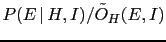
- ... as62
-
Factorizing
 and
and
 respectively
in the numerator and in the denominator, Eq. (39)
becomes
respectively
in the numerator and in the denominator, Eq. (39)
becomes
Then
 can be indicated as
 ,
,
 is equal to
 and, finally,
can be written as
and, finally,
can be written as
 .
.
.
.
.
.
.
.
.
.
.
.
.
.
.
.
.
.
.
.
.
.
.
.
.
.
.
.
.
.
.
.
- ...condition63
- Otherwise, obviously
 cannot be factorized.
The effective odds
cannot be factorized.
The effective odds
 can
however be written in the following convenient forms
can
however be written in the following convenient forms
although less interesting than Eq. (41).
.
.
.
.
.
.
.
.
.
.
.
.
.
.
.
.
.
.
.
.
.
.
.
.
.
.
.
.
.
.
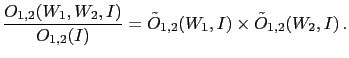
- ... network,64
- In complex situations
an effects might have several (con-)causes; or
an effect can be itself a cause of other effects;
and so on. As it can be easily imagined,
causes and effects can be represented by a graph,
as that of figure 2.
Since the connections between the nodes
of the resulting network have usually the meaning
of probabilistic links (but also deterministic relations
can be included), this graph is called a belief network.
Moreover, since Bayes' theorem is used to update the probabilities
of the possible states of the nodes (the node `Box',
with reference to our toy model, has states and ;
the node `Ball' has states
 and ), they are also
called Bayesian networks.
For more info, as well as tutorials and demos
of powerful packages having
also a friendly graphical user interface,
I recommend visiting Hugin [12] and
Netica [13] web sites.
(My preference for Hugin is mainly due to the fact that
it is multi-platform and runs nicely under Linux.)
For a book
introducing Bayesian networks in forensics, Ref. [14]
is recommended. For a monumental
probabilistic network on the `case that will never end',
see Ref. [15]
(if you like classic thrillers,
the recent paper of the same author might be of your interest
[16]).
and ), they are also
called Bayesian networks.
For more info, as well as tutorials and demos
of powerful packages having
also a friendly graphical user interface,
I recommend visiting Hugin [12] and
Netica [13] web sites.
(My preference for Hugin is mainly due to the fact that
it is multi-platform and runs nicely under Linux.)
For a book
introducing Bayesian networks in forensics, Ref. [14]
is recommended. For a monumental
probabilistic network on the `case that will never end',
see Ref. [15]
(if you like classic thrillers,
the recent paper of the same author might be of your interest
[16]).
.
.
.
.
.
.
.
.
.
.
.
.
.
.
.
.
.
.
.
.
.
.
.
.
.
.
.
.
.
.
- ... factors'.65
- Note that there are in general two lie factors,
one for and one for
 . For simplicity we assume here
they have the same value.
. For simplicity we assume here
they have the same value.
.
.
.
.
.
.
.
.
.
.
.
.
.
.
.
.
.
.
.
.
.
.
.
.
.
.
.
.
.
.
- ... us66
- The Hugin file
can be found in
http://www.roma1.infn.it/~dagos/prob+stat.html#Columbo.
.
.
.
.
.
.
.
.
.
.
.
.
.
.
.
.
.
.
.
.
.
.
.
.
.
.
.
.
.
.
![$\displaystyle \left\{\begin{array}{rcl} \mbox{E}[\Delta\mbox{JL}_{1,2}(H_1)] &=...
...4
\\
u_R[\Delta\mbox{JL}_{1,2}(H_1)] &=& 1.6
\end{array}\right.
\hspace{0.5cm}$](img409.png)
![$\displaystyle \hspace{0.5cm}
\left\{\begin{array}{rcl} \mbox{E}[\Delta\mbox{JL}...
...1,2}(H_2)]&=&0.97
\\
u_R[\Delta\mbox{JL}_{1,2}(H_2)] &=&2.6
\end{array}\right.$](img410.png)
 JL
JL