Introduction

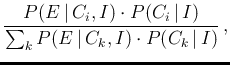
As it is becoming rather well known, the only sound way to solve what Poincaré called “the essential problem of the experimental method” is to tackle it using probability theory, as it should be rather obvious for “a problem in the probability of causes”. The mathematical tool to perform what is also known as `probability inversion' is called Bayes rule (or theorem), although due to Laplace, at least in one of the most common formulations:¹

$$P(C_i\,\vert\,E,I) = \frac{P(E\,\vert\,C_i,I)\cdot P(C_i\,\vert\,I)} {\sum_k P(E\,\vert\,C_k,I)\cdot P(C_k\,\vert\,I)}\,, % =$$ (1)

where $E$ is the observed event and $C_i$ are its possible causes, forming a complete class (i.e. exhaustive and mutually exclusive). `$I$' stands for the background state of information, on which all probability evaluations do depend (`$I$' is often implicit, as it will be later in this paper, but it is important to remember of its existence).

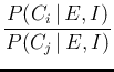
Considering also an alternative cause $C_j$, the ratio of the two posterior probabilities, that is how the two hypotheses are re-ranked in degree of belief, in the light of the observation $E$, is given by

$$\frac{P(C_i\,\vert\,E,I)}{P(C_j\,\vert\,E,I)} = \frac{P(E\,\vert\,C_i,I)}{P(E\,\vert\,C_j,I)} \times \frac{P(C_i\,\vert\,I)}{P(C_j\,\vert\,I)}\,,$$ (2)

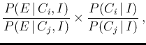
in which we have factorized the r.h. side into the initial ratio of probabilities of the two causes (second term) and the updating factor

$$\frac{P(E\,\vert\,C_i,I)}{P(E\,\vert\,C_j,I)}\,,$$ (3)

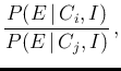
known as Bayes factor, or `likelihood ratio'.<sup>2</sup>The advantage of Eq. (2) with respect to Eq. (1) is that it highlights the two contributions to the posterior ratio of the hypothesis of interest: the prior probabilities of the `hypotheses', on which there could be a large variety of opinions; the ratio of the probabilities of the observed event, under the assumption to each hypothesis of interest, which can often be rather intersubjective, in the sense that there is usually a larger, or unanimous consensus, if the conditions under they have been evaluated (`$I$') are clearly stated and shared (and in critical cases we have just to rely on the well argued and documented opinion of experts.³)

Recently, going after years through the third section of the second `book' of Gauss' Theoria motus corporum coelestium in sectionibus conicis solem ambientum [7,8], of which I had read with the due care only the part in which the Prince Mathematicorum derives in his peculiar way what is presently known as the Gaussian (or `normal') error function, I have realized that Gauss had also illustrated, a few pages before, a theorem on how to update the probability ratio of two alternative hypotheses, based on experimental observations. Indeed the theorem is not exactly Eq.(2), because it is only formulated for the case in which $P(C_i\,\vert\,I)$ and $P(C_j\,\vert\,I)$ are equal, but the reasoning Gauss had setup would have led naturally to the general case. It seems that he focused into the sub-case of a priori equally likely hypotheses just because he had to apply his result to a problem in which he consider the values to be inferred a priori equally likely (“valorum harum incognitarum ante illa observationes aeque probabilia fuisse”).

But let us proceed in order.