P-value based on the argument that the highest excess could have shown up everywhere in the time distribution

Again, the previous procedure can be easily criticized, because ``the bin to which the test has been applied has been chosen after having observed the data, while a peak would have been arisen, a priori, everywhere in the plot.'' The standard procedure to overcome this criticism is to calculate the probability that a peak of that or higher value would have shown up everywhere in the data, i.e.

$$\left.\mbox{p-value}\right\vert _{\mbox{scan}} = 1-\prod_{i=1}^{n_{bin}} F(3\,\vert\,{\cal P}_{\lambda_B})\,,$$ (3)

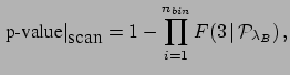where $n_{bin}$ is the number of bins and $F(\cdot)$ stands for the cumulative distribution (the product in Eq. (3) is based on the assumption of independence of the bins). In our case we get 13% or 23% depending whether a constant or varying background is assumed, i.e. p-values above any over-optimistic choice of the p-value threshold.

It is interesting to note that the $13\%$ p-value can be reobtained approximately as $\left.\mbox{p-value}\right\vert _{\mbox{scan}} \approx n_{bin}\times \left.\mbox{p-value}\right\vert _{\mbox{max}}$, showing that even a very pronounced excess can be considered not significant if a large number of observational bins are involved in the experiment (and practitioners restrict arbitrary the region to which the test is applied, if they want the test to state what they would like...). The dependence of the result of the method on observations far from the region where there could be a good physical reason to have a signal is annoying (and for this reason, practitioners who choose a suitable region around the peak do, intuitively, something correct...). On the other hand, the reasoning does not take into account that other bins could be interested by the signal.

We shall see in Sec. 4.3 how to use properly the prior knowledge that a (physically motivated) signal could have appeared everywhere in the histogram.