Next: Models for Galactic sources
Up: Bayesian model comparison applied
Previous: Why not to use
The Bayesian way out: how to use of experimental data
to update the credibility of hypotheses
We think that the solution to the above problems consists
in changing radically our attitude, instead of seeking for
new `prescriptions' which might cure a trouble but generate others.
The so called Bayesian approach, based on the natural idea
of probability as `degree of belief' and on the rules of logic,
seems to us to be the proper way to deal with our problem.
A key role in this approach is played by Bayes' theorem,
which, apart from normalization constant, can be stated as
where  stand the hypotheses that could
produce the Data with likelihood
stand the hypotheses that could
produce the Data with likelihood
 Data
Data
 .
.
 Data
Data and
and
 are, respectively,
the posterior and prior probabilities, i.e. with or
without taking into account
the information provided by the Data.
are, respectively,
the posterior and prior probabilities, i.e. with or
without taking into account
the information provided by the Data.  stands
for the general status of information,
which is usually considered implicit
and will then be omitted in the following formulae.
stands
for the general status of information,
which is usually considered implicit
and will then be omitted in the following formulae.
The presence of priors, considered a weak point by opposer's
of the Bayesian theory, is one of the points of force of the theory.
First, because priors are necessary to make the `probability
inversion' of Eq. (4).
Second, because in this approach all relevant conditions must be clearly stated,
instead of being hidden in the method or left to the arbitrariness
of the practitioner. Third, because prior knowledge can be properly
incorporated in the analysis to integrate missing or deteriorated
experimental information (and whatever it is done should be
stated explicitly!). Finally, because the clear separation
of prior and likelihood in Eq. (4) allows to
publish the results in a way independent from
,
if the priors might differ largely within the members of the
scientific community. In particular, the Bayes factor,
defined as
 |
(5) |
is the factor which changes the `bet odds' (i.e. probability ratios)
in the light of the new data. In fact, dividing member to member
Eq. (4) written for hypotheses and  , we get
posterior odds prior odds prior odds |
(6) |
Since we shall speak later about models
 , the odd ratio updating is given
by
, the odd ratio updating is given
by
 |
(7) |
Some general remarks are in order.
- Conclusions depend only on the observed data and on the previous knowledge.
In particular they do not depend on unobserved data which are rarer than the
data really observed (that is what p-values imply).
- At least two models have to be taken into account, and the likelihood
for each model must be specified.
- There is no need to consider `all possible models',
since what matters are relative beliefs.
- Similarly, there is no need that the model must be declared before the data
are taken, or analyzed.
What matters is that the initial beliefs should be based on general
arguments about the plausibility of each model and on agreement with
other experimental information,
other than Data.
An analogue of Eq. (4) applies to the parameters of a model.
For example, if, given a model 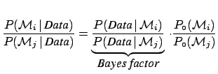 , we are interested to the
rate of g.w. on Earth,
, we are interested to the
rate of g.w. on Earth,  , Bayes' theorem gives
 |
(8) |
where 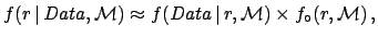 stand for probability density functions (pdf)
Also in this case, a prior independent way of reporting the result
is possible. The difficulty
of dealing with an infinite number of Bayes factors
(precisely
stand for probability density functions (pdf)
Also in this case, a prior independent way of reporting the result
is possible. The difficulty
of dealing with an infinite number of Bayes factors
(precisely  , given each
  and
and  ) can be overcome
defining a function
) can be overcome
defining a function  of which gives the Bayes factor with
respect to a reference
of which gives the Bayes factor with
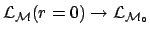
respect to a reference  . This function is particularly
useful if is chosen to be the asymptotic value
at which the experiment looses completely sensitivity.
For g.w. search this asymptotic value is simply
. This function is particularly
useful if is chosen to be the asymptotic value
at which the experiment looses completely sensitivity.
For g.w. search this asymptotic value is simply
 .
In other cases it could be an infinite particle mass [3]
or an infinite mass scale [4]. In the case of g.w. rate ,
extensively discussed in Ref. [5], we get
.
In other cases it could be an infinite particle mass [3]
or an infinite mass scale [4]. In the case of g.w. rate ,
extensively discussed in Ref. [5], we get
 |
(9) |
where
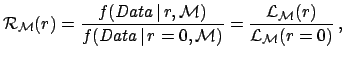 is the model dependent likelihood.
[Note that, indeed, in the limit of
the likelihood depends
only on the background expectation and not on the specific model. Therefore
is the model dependent likelihood.
[Note that, indeed, in the limit of
the likelihood depends
only on the background expectation and not on the specific model. Therefore
 , where
 stands for the model ``background alone''.]
This function has the meaning of
relative belief updating factor [5],
since it tells us how we must modify our beliefs of the
different values of , given the observed data. In the region
where vanishes, the corresponding values of are excluded.
On the other hand, in the region where is about unity,
the data are unable to change our beliefs, i.e. we have lost sensitivity.
The region of transition between 0 and 1 defines the
sensitivity bound, a concept that does not have a probabilistic
meaning and, since it does not refers to terms such as `confidence',
does not cause the typical misinterpretations of the frequentistic
`confidence upper/lower limits' (for a recent example of
results using these ideas see Ref. [8]).
Values of preferred by the data are spotted by large value of .
We shall in the sequel how a plot of the function gives
an immediate representation of what the data tell about a parameter
(Figs. 3 and 4).
Another interesting feature of this function is that, if several
independent data sets are available, each providing some information
about model , the global information is obtained multiplying
the various functions:
stands for the model ``background alone''.]
This function has the meaning of
relative belief updating factor [5],
since it tells us how we must modify our beliefs of the
different values of , given the observed data. In the region
where vanishes, the corresponding values of are excluded.
On the other hand, in the region where is about unity,
the data are unable to change our beliefs, i.e. we have lost sensitivity.
The region of transition between 0 and 1 defines the
sensitivity bound, a concept that does not have a probabilistic
meaning and, since it does not refers to terms such as `confidence',
does not cause the typical misinterpretations of the frequentistic
`confidence upper/lower limits' (for a recent example of
results using these ideas see Ref. [8]).
Values of preferred by the data are spotted by large value of .
We shall in the sequel how a plot of the function gives
an immediate representation of what the data tell about a parameter
(Figs. 3 and 4).
Another interesting feature of this function is that, if several
independent data sets are available, each providing some information
about model , the global information is obtained multiplying
the various functions:
Subsections
Next: Models for Galactic sources
Up: Bayesian model comparison applied
Previous: Why not to use
Giulio D'Agostini
2005-01-09