 |
(52) | ||
 |
(53) | ||
 |
(54) |
 |
(55) |
Other interesting limit cases are the following.
The prior
![]() has been left on purpose open
in the above
formulas, although we have already anticipated that usually a flat
prior about all parameters gives the correct result in most 'healthy'
cases, characterized by a sufficient number of data points.
I cannot go here through an extensive discussion about the
issue of the priors, often criticized as the weak point of the Bayesian
approach and that are in reality one of its points of force. I refer
to more extensive discussions available elsewhere (see e.g. [2]
and references therein), giving here only a couple of advices.
A flat prior is in most times a good starting point (unless
one uses some packages, like BUGS [11], that does not like
flat prior in the range
has been left on purpose open
in the above
formulas, although we have already anticipated that usually a flat
prior about all parameters gives the correct result in most 'healthy'
cases, characterized by a sufficient number of data points.
I cannot go here through an extensive discussion about the
issue of the priors, often criticized as the weak point of the Bayesian
approach and that are in reality one of its points of force. I refer
to more extensive discussions available elsewhere (see e.g. [2]
and references therein), giving here only a couple of advices.
A flat prior is in most times a good starting point (unless
one uses some packages, like BUGS [11], that does not like
flat prior in the range ![]() to
to ![]() ; in this case
one can mimic it with a very broad distribution, like a
Gaussian with very large
; in this case
one can mimic it with a very broad distribution, like a
Gaussian with very large ![]() ).
If the result of the inference `does not offend your physics
sensitivity', it means that, essentially, flat priors have done a good
job and it is not worth fooling around with more sophisticated ones.
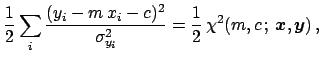
In the specific case we are looking closer, that of
Eq. (53),
the most critical quantity to watch is obviously
).
If the result of the inference `does not offend your physics
sensitivity', it means that, essentially, flat priors have done a good
job and it is not worth fooling around with more sophisticated ones.
In the specific case we are looking closer, that of
Eq. (53),
the most critical quantity to watch is obviously ![]() , because
it is positively defined. If, starting from a flat prior
(also allowing negative values),
the data constrain the value of
, because
it is positively defined. If, starting from a flat prior
(also allowing negative values),
the data constrain the value of ![]() in a (positive) region far from zero,
and - in practice consequently -
its marginal distribution is approximatively
Gaussian, it means the flat prior was a reasonable choice.
Otherwise, the next-to-simple modeling of
in a (positive) region far from zero,
and - in practice consequently -
its marginal distribution is approximatively
Gaussian, it means the flat prior was a reasonable choice.
Otherwise, the next-to-simple modeling of ![]() is via
the step function
is via
the step function
![]() . A more technical choice
would be a gamma distribution, with suitable parameters
to `easily' accommodate all envisaged values of
. A more technical choice
would be a gamma distribution, with suitable parameters
to `easily' accommodate all envisaged values of ![]() .
.
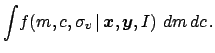
The easiest case, that happens very often if one has `many' data points
(where `many' might be already as few as some dozens),
is that
![]() obtained starting from flat priors
is approximately a multi-variate Gaussian distribution,
i.e. each marginal is approximately Gaussian.
In this case the expected value of each variable is
close to its mode, that, since the prior was a constant,
corresponds to the value for which the likelihood
obtained starting from flat priors
is approximately a multi-variate Gaussian distribution,
i.e. each marginal is approximately Gaussian.
In this case the expected value of each variable is
close to its mode, that, since the prior was a constant,
corresponds to the value for which the likelihood
![]() gets its maximum.
Therefore the parameter estimates derived by the
maximum likelihood principle are very good approximations
of the expected values of the parameters calculated directly
from
gets its maximum.
Therefore the parameter estimates derived by the
maximum likelihood principle are very good approximations
of the expected values of the parameters calculated directly
from
![]() . In a certain sense the maximum likelihood
principle best estimates are recovered as a special case that holds
under particular conditions (many data points and vague priors).
If either condition fails, the result
the formulas derived from such a principle
might be incorrect.
This is the reason I dislike unneeded principles of this
kind, once we have a more general framework, of which the
methods obtained by `principles' are just special cases under well
defined conditions.
. In a certain sense the maximum likelihood
principle best estimates are recovered as a special case that holds
under particular conditions (many data points and vague priors).
If either condition fails, the result
the formulas derived from such a principle
might be incorrect.
This is the reason I dislike unneeded principles of this
kind, once we have a more general framework, of which the
methods obtained by `principles' are just special cases under well
defined conditions.
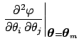
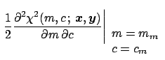
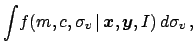
The simple case in which
![]() is approximately
multi-variate Gaussian allows also to approximately
evaluate the covariance matrix of the fit parameters from
the Hessian of its logarithm.6This is due to a well known
property of the multi-variate Gaussian and it is not strictly
related to flat priors.
In fact it can easily proved that if the generic
is approximately
multi-variate Gaussian allows also to approximately
evaluate the covariance matrix of the fit parameters from
the Hessian of its logarithm.6This is due to a well known
property of the multi-variate Gaussian and it is not strictly
related to flat priors.
In fact it can easily proved that if the generic
![]() is a multivariate Gaussian, then
is a multivariate Gaussian, then
| (62) |
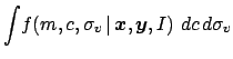
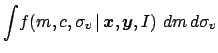
An interesting feature of this approximated procedure is that,
since it is based on the logarithm of the pdf, normalization factors
are irrelevant. In particular, if the priors are flat, the
relevant summaries of the inference
can be obtained from the logarithm of the likelihood, stripped
of all irrelevant factors (that become additive constants
in the logarithm and vanish in the derivatives).
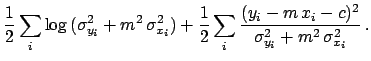
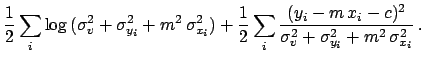
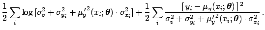
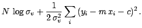
Let us write down, for some cases of interest,
the minus-log-likelihoods, stripped of constant terms
and indicated by ![]() , i.e.
, i.e.
![]() .
.
 |
(66) |
![$\displaystyle k\, \prod_i
\frac{1}{\sqrt{\sigma^2_v + \sigma_{y_i}^2+m^2\,\sigm...
...+ \sigma_{y_i}^2+m^2\,\sigma_{x_i}^2) }
\right]}\, f(m,c,\sigma_v\,\vert\,I)\,,$](img174.png)
![$\displaystyle \prod_i
\exp{ \left[ -\frac{(y_i-m\,x_i-c)^2}
{2\, \sigma_{y_i}^2}
\right]}\, f(m,c\,\vert\,I)$](img187.png)
![$\displaystyle \exp{ \left[-\frac{1}{2}\sum_i \frac{(y_i-m\,x_i-c)^2}
{\sigma_{y_i}^2} \right]}\, f(m,c\,\vert\,I) \,.$](img188.png)
![$\displaystyle \prod_i
\frac{1}{\sqrt{\sigma^2_v + \sigma_{y_i}^2}}\,
\exp{ \lef...
...2}
{2\, (\sigma^2_v + \sigma_{y_i}^2) }
\right]}\, f(m,c,\sigma_v\,\vert\,I)\,.$](img189.png)
![$\displaystyle \sigma_v^{-N} \prod_i
\exp{ \left[ -\frac{(y_i-m\,x_i-c)^2}
{2\,\sigma^2_v }
\right]}\, f(m,c,\sigma_v\,\vert\,I)$](img190.png)
![$\displaystyle \sigma_v^{-N}
\exp{ \left[
-\frac{1}{2\,\sigma_v^2} \,\sum_i (y_i-m\,x_i-c)^2
\right]}\, f(m,c,\sigma_v\,\vert\,I)
\,.$](img191.png)