Predicting numbers of counts, their difference and their ratio
The Poisson distribution hardly needs any introduction,
beside, perhaps, that it can be framed within the
Poisson process,
which has indeed its roots in the Bernoulli process.
This picture makes the Poissonian related
to other important distributions,
as reminded in Appendix A, which can be seen as a
technical preface to the paper.
Using the notation introduced there,
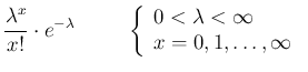
the Poisson probability function is given by2
and it quantifies how much we believe that  counts will occur,
if we assume an exact value of the parameter
counts will occur,
if we assume an exact value of the parameter
 .3As well known,
expected value and standard deviation of
.3As well known,
expected value and standard deviation of  are and
 . The most probable value
of (`mode') is equal to the integer just below
(`floor
. The most probable value
of (`mode') is equal to the integer just below
(`floor ') in the case is not integer.
Otherwise is equal to itself, and also to
') in the case is not integer.
Otherwise is equal to itself, and also to  (remember that cannot be null).
If we have two independent Poisson distributions
characterized
by  and
and  , i.e.
we `expect' their difference
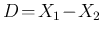 `to be'
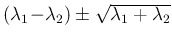 ,
as it results from well known theorems of probability
theory4(hereafter, unless indicated otherwise, the notation
`
,
as it results from well known theorems of probability
theory4(hereafter, unless indicated otherwise, the notation
`
 ' stands for `expected value of the quantity
  its standard uncertainty' [9],
that is the standard deviation of the associated probability distribution).
its standard uncertainty' [9],
that is the standard deviation of the associated probability distribution).
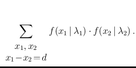
The probability distribution of  can be obtained
`from the inventory of the values of
can be obtained
`from the inventory of the values of  and
and  that result
in each possible value of ', that is
that result
in each possible value of ', that is
For example, in the case of
 ,
the most probable contributions to are shown
in Tab.
,
the most probable contributions to are shown
in Tab. ![[*]](crossref.png) .
.
Table:
Table of the most probable differences
for
 (probability of each entry in the table
within square brackets).
(probability of each entry in the table
within square brackets).
|
|
|
|
|
|
|
0 |
1 |
2 |
3 |
4 |
5 |
|
|
0 |
0 |
-1 |
-2 |
-3 |
-4 |
-5 |
|
|
|
[0.135335] |
[0.135335] |
[0.067668] |
[0.022556] |
[0.005639] |
[0.001128] |
|
|
1 |
1 |
0 |
-1 |
-2 |
-3 |
-4 |
|
|
|
[0.135335] |
[0.135335] |
[0.067668] |
[0.022556] |
[0.005639] |
[0.001128] |
|
|
2 |
2 |
1 |
0 |
-1 |
-2 |
-3 |
|
|
|
[0.067668] |
[0.067668] |
[0.033834] |
[0.011278] |
[0.002819] |
[0.000564] |
|
|
3 |
3 |
2 |
1 |
0 |
-1 |
-2 |
|
|
|
[0.022556] |
[0.022556] |
[0.011278] |
[0.003759] |
[0.000940] |
[0.000188] |
|
|
4 |
4 |
3 |
2 |
1 |
0 |
-1 |
|
|
|
[0.005639] |
[ 0.005639] |
[0.002819] |
[0.000940] |
[0.000235] |
[0.000047] |
|
|
5 |
5 |
4 |
3 |
2 |
1 |
0 |
|
|
|
[0.001128] |
[0.001128] |
[0.000564] |
[0.000188] |
[0.000047] |
[0.000009]
|
|
For instance, the probability to get  sums up to 30.9%.
The probability decreases
symmetrically for larger absolute values of the difference.
Without entering into the question of getting
a closed form of
sums up to 30.9%.
The probability decreases
symmetrically for larger absolute values of the difference.
Without entering into the question of getting
a closed form of
 ,5
it can be instructive to implement
Eq. (), although in an approximate
and rather inefficient way, in
a few lines of R code [11]:6
,5
it can be instructive to implement
Eq. (), although in an approximate
and rather inefficient way, in
a few lines of R code [11]:6
dPoisDiff <- function(d, lambda1, lambda2) {
   xmax = round(max(lambda1,lambda2)) + 20*sqrt(max(lambda1,lambda2))
   sum( dpois((0+d):xmax, lambda1) * dpois(0:(xmax-d), lambda2) )
}
This function is part of the code provided in Appendix B.1,
which produces the plot of Fig. ,
evaluating also expected value and standard deviation
(indeed approximated values, being xmax not too large).
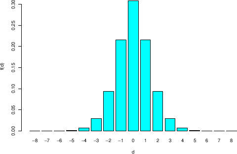
Figure:
Distribution of the difference of counts
resulting from two Poisson distributions with
.
 |
Moving to the ratio of counts, numerical problems might arise,
as shown in Tab. , analogue of Tab. .
Table:
Table of the most probable ratios  for
.
`NaN' and `Inf' are the R symbols
for undefined (`not a number') and infinity, resulting from
a vanishing denominator.
for
.
`NaN' and `Inf' are the R symbols
for undefined (`not a number') and infinity, resulting from
a vanishing denominator.
|
|
|
|
|
|
|
0 |
1 |
2 |
3 |
4 |
5 |
|
|
0 |
red NaN |
0 |
0 |
0 |
0 |
0 |
|
|
|
[ red0.135335] |
[0.135335] |
[0.067668] |
[0.022556] |
[0.005639] |
[0.001128] |
|
|
1 |
red Inf |
1 |
1/2 |
1/3 |
1/4 |
1/5 |
|
|
|
[red 0.135335] |
[0.135335] |
[0.067668] |
[0.022556] |
[0.005639] |
[0.001128] |
|
|
2 |
red Inf |
2 |
1 |
2/3 |
1/2 |
2/5 |
|
|
|
[red 0.067668] |
[0.067668] |
[0.033834] |
[0.011278] |
[0.002819] |
[0.000564] |
|
|
3 |
red Inf |
3 |
3/2 |
1 |
3/4 |
3/5 |
|
|
|
[red 0.022556] |
[0.022556] |
[0.011278] |
[0.003759] |
[0.000940] |
[0.000188] |
|
|
4 |
red Inf |
4 |
2 |
4/3 |
1 |
4/5 |
|
|
|
[red 0.005639] |
[ 0.005639] |
[0.002819] |
[0.000940] |
[0.000235] |
[0.000047] |
|
|
5 |
red Inf |
5 |
5/2 |
5/3 |
5/4 |
1 |
|
|
|
[red 0.001128] |
[0.001128] |
[0.000564] |
[0.000188] |
[0.000047] |
[0.000009]
|
|
In fact for rather small values of
there is high chance
(exactly the probability of getting  )
that the ratio results in
an undefined form or an infinite, reported
in the table using the R symbols NaN (`not a number')
and Inf, respectively.
As we can see,
we have now quite a variety of possibilities
and the probability distribution of the ratios
is rather irregular. For this reason, in this case
we evaluate it by Monte Carlo methods using R.7Figure
)
that the ratio results in
an undefined form or an infinite, reported
in the table using the R symbols NaN (`not a number')
and Inf, respectively.
As we can see,
we have now quite a variety of possibilities
and the probability distribution of the ratios
is rather irregular. For this reason, in this case
we evaluate it by Monte Carlo methods using R.7Figure
Figure:
Monte Carlo distribution of the ratio of counts
resulting from two Poisson distributions with
 .
.
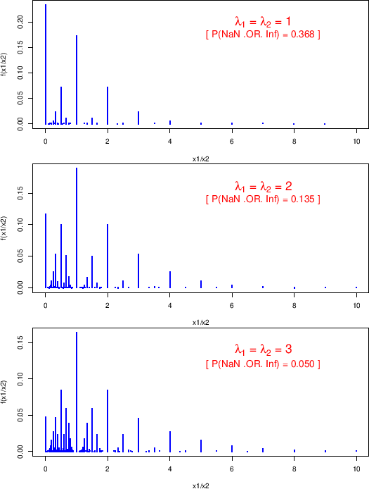 |
shows the distributions
of the ratio for
 .
The figure also reports the probability to get an infinite
or an undefined expression, equal to
.
The figure also reports the probability to get an infinite
or an undefined expression, equal to
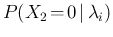 .
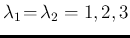
When is very large the probability to get ,
and therefore of being equal to Inf or NaN, vanishes.
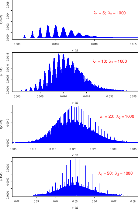
But the distribution of the ratio remains quite `irregular', if looked
into detail, even for `not so small', as
shown in Fig. for the cases
of
.
When is very large the probability to get ,
and therefore of being equal to Inf or NaN, vanishes.
But the distribution of the ratio remains quite `irregular', if looked
into detail, even for `not so small', as
shown in Fig. for the cases
of
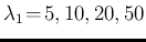 and
and
 .
.
Figure:
Monte Carlo distribution of the ratio of counts
resulting from two Poisson distributions with
 and
and
 .
.
 |
However we should not be worried about
this kind of distributions, which are not more than entertaining
curiosities, as long as physics questions are concerned. Why should
we be interested in the ratio of counts that we might observe
for different 's? If we want to get an idea of how
much the counts could differ, we can just use the probability
distribution of their possible differences, which has a regular behavior,
without divergences or undefined forms.
The deep reason
for speculating about “ratios of small numbers of events”
and their “errors”[3] is due
to a curious ideology at the basis of a school of Statistics
which limits the applications of Probability Theory.
Indeed, we, as physicists,
are often interested in the ratio of the rates of
Poisson processes, that is in
 , being
this quantity related to some physical quantities having
a theoretical relevance.
Therefore we aim to learn
which values of
, being
this quantity related to some physical quantities having
a theoretical relevance.
Therefore we aim to learn
which values of  are more or less probable in the light
of the experimental observations. Stated in this terms,
we are interested in evaluating `somehow' (not always in closed form)
the probability density function (pdf)
are more or less probable in the light
of the experimental observations. Stated in this terms,
we are interested in evaluating `somehow' (not always in closed form)
the probability density function (pdf)
 ,
given the observations of
,
given the observations of  counts during
  and
of
and
of  counts during
  (and also conditioned
on the background state of
knowledge, generically indicated by
(and also conditioned
on the background state of
knowledge, generically indicated by  ).
But there are statisticians who maintain that we can only talk about
the probability of counts, assuming , and
not of the probability distribution
of having observed
).
But there are statisticians who maintain that we can only talk about
the probability of counts, assuming , and
not of the probability distribution
of having observed  , and even less
of
, and even less
of
 (same as
  , if
, if
 )
having observed and counts.8
)
having observed and counts.8
If, instead, we follow an approach closer to that innate
in the human mind, which naturally attaches the concept of probability to
whatever is considered uncertain [16],
there is no need to go through contorted reasoning.
For example,
if we observe  , then we tend to believe that this effect
has been caused
more likely by a value of around 1 rather than around 10 or 20, or larger,
although
we cannot rule out with certainty such values.
Similarly, sticking to the observation of ,
we tend to believe to
, then we tend to believe that this effect
has been caused
more likely by a value of around 1 rather than around 10 or 20, or larger,
although
we cannot rule out with certainty such values.
Similarly, sticking to the observation of ,
we tend to believe to
 much more
than to
much more
than to
 , or smaller.
In particular,
, or smaller.
In particular,  is definitely ruled out,
because it could only yield 0 counts (this is just a limit case,
since the Poisson is defined positive).
is definitely ruled out,
because it could only yield 0 counts (this is just a limit case,
since the Poisson is defined positive).
It is then clear that, as far as the ratio
of
is concerned, there are
no divergences, no matter how small the numbers
of counts might be, obviously with two exceptions.
The first is when is observed to be exactly 0 (but in this case
we could turn our interest in
 ,
assuming
,
assuming  ). The second is
when is not zero, but there could be some background,
such that
). The second is
when is not zero, but there could be some background,
such that  is not excluded with certainty [13,17].
The effect of possible background is not going to be treated
in detail in this paper,
and only some hints on how to include it into the model
will be given.
is not excluded with certainty [13,17].
The effect of possible background is not going to be treated
in detail in this paper,
and only some hints on how to include it into the model
will be given.