- ...
imperfect.1
- This problem has been treated
in much detail in Ref. [1],
taking cue from questions related to the Covid-19 pandemic.
.
.
.
.
.
.
.
.
.
.
.
.
.
.
.
.
.
.
.
.
.
.
.
.
.
.
.
.
.
.
- ... by2
- I try,
whenever it is possible,
to stick to the convention
of capital letters for the name of a variable
and small letters for its possible values.
Exceptions are Greek letters and quantities
naturally defined by a small letter, like
 for a `rate'.
.
.
.
.
.
.
.
.
.
.
.
.
.
.
.
.
.
.
.
.
.
.
.
.
.
.
.
.
.
.
- ....3
- If, instead, we are uncertain about
 and quantify its uncertainty by the probability density function
 , where
  stands for our status
of information about that quantity, the distribution of the counts
will be given by
stands for our status
of information about that quantity, the distribution of the counts
will be given by
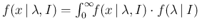 d
d
.
.
.
.
.
.
.
.
.
.
.
.
.
.
.
.
.
.
.
.
.
.
.
.
.
.
.
.
.
.
- ...
theory4
- In brief: the expected value of a linear combination
is the linear combination of the expected values;
the variance of a linear combination is the linear combination
of the variances, with squared coefficients.
.
.
.
.
.
.
.
.
.
.
.
.
.
.
.
.
.
.
.
.
.
.
.
.
.
.
.
.
.
.
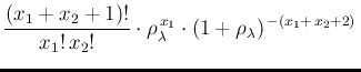
- ...,5
- Such a distribution is known in
the literature as Skellam distribution [10] and
it is available in R [11] installing the
homonym package [12].
The distribution of the differences corresponding to the cases of
Tab.
![[*]](crossref.png) can be easily plotted by the
following R commands, producing a bar plot similar to that
of Fig. ,
can be easily plotted by the
following R commands, producing a bar plot similar to that
of Fig. ,
  library(skellam)
  d = -5:5
  barplot(dskellam(d,1,1), names=d, col='cyan')
.
.
.
.
.
.
.
.
.
.
.
.
.
.
.
.
.
.
.
.
.
.
.
.
.
.
.
.
.
.
- ...R:6
- This function,
hopefully having a didactic value, is not
optimized at all and it uses the fact that the R function
dpois() returns zero for negative values of the
variable.
.
.
.
.
.
.
.
.
.
.
.
.
.
.
.
.
.
.
.
.
.
.
.
.
.
.
.
.
.
.
- ... R.7
- The
core of the R code is given,
for the case of
 , by
, by
lambda1 = lambda2 = 1; n = 10^6
x1 = rpois(n,lambda1)
x2 = rpois(n,lambda2)
rx = x1/x2
rx = rx[!is.nan(rx) & (rx != Inf)]
barplot(table(rx)/n, col='cyan', xlab='x1/x2', ylab='f(x1/x2)')
.
.
.
.
.
.
.
.
.
.
.
.
.
.
.
.
.
.
.
.
.
.
.
.
.
.
.
.
.
.
- ... counts.8
- Ref. [3]
is a kind of `masterpiece' of the kind of convoluted reasoning involved.
For example, the paper starts with the following incipit
(quote marks original):
When the result of the measurement of a physical quantity
is published as
 without further explanation, it is
implied that
without further explanation, it is
implied that  is a gaussian-distributed measurement with mean
  and variance
 . This allows one to calculate
various confidence intervals of given “probability”,
i.e., the “probability”
. This allows one to calculate
various confidence intervals of given “probability”,
i.e., the “probability”  that the true value of is within
a given interval.
that the true value of is within
a given interval.
However, nowhere in the paper is explained why probability
is within quote marks. The reason is simply because the authors
are fully aware that frequentist ideology, to which they overtly
adhere, refuses to attach the concept of probability to
true values, as well as to model parameters, and so on
(see e.g. Ref. [13]). But authoritative statements of this
kind might contribute to increase the confusion of
practitioners [14], who then tend to take
frequentist `confidence levels' as if they were
probability values [15].
.
.
.
.
.
.
.
.
.
.
.
.
.
.
.
.
.
.
.
.
.
.
.
.
.
.
.
.
.
.
- ...
`prior'.9
- This name is somehow unfortunate, because
it might induce people think to time order, as discussed
in Ref. [1], in which it is shown how,
instead, the `prior' can be applied in a second step,
in particular by someone else, if a `flat prior' used.
.
.
.
.
.
.
.
.
.
.
.
.
.
.
.
.
.
.
.
.
.
.
.
.
.
.
.
.
.
.
- ...fig:pdf_lambda_x1_x2_MC_high.10
- The
complete script is provided in Appendix B.2.
.
.
.
.
.
.
.
.
.
.
.
.
.
.
.
.
.
.
.
.
.
.
.
.
.
.
.
.
.
.
- ... value”11
- For
the reason of the quote marks see footnote .
.
.
.
.
.
.
.
.
.
.
.
.
.
.
.
.
.
.
.
.
.
.
.
.
.
.
.
.
.
.
- ...fig:pdf_lambda_x1_x2_MC_high,12
- Zero overflow
in that plot is only due to the `limited' number of sampled,
chosen to be
 , and to the fact that the same script
of the other plot has been used.
, and to the fact that the same script
of the other plot has been used.
.
.
.
.
.
.
.
.
.
.
.
.
.
.
.
.
.
.
.
.
.
.
.
.
.
.
.
.
.
.
- ...eq:sommatoria),13
- for a different
approach to get Eq. ()
see footnote ,
in which the integrand of Eq. ()
is interpreted as the joint pdf of
 ,
,  and
and  .
.
.
.
.
.
.
.
.
.
.
.
.
.
.
.
.
.
.
.
.
.
.
.
.
.
.
.
.
.
.
.
- ... integrals14
- Work
done on a Raspberry Pi3, thanks to Mathematica 12.0 generously
offered by Wolfram Inc. to the Raspbian system.
.
.
.
.
.
.
.
.
.
.
.
.
.
.
.
.
.
.
.
.
.
.
.
.
.
.
.
.
.
.
- ....15
- To be precise,
the condition is
 and
and  , but, given the role of the two variables in our context,
it means for all possible counts (including
, but, given the role of the two variables in our context,
it means for all possible counts (including
 , for which the pdf becomes
 , having
however infinite mean and variance.)
, having
however infinite mean and variance.)
.
.
.
.
.
.
.
.
.
.
.
.
.
.
.
.
.
.
.
.
.
.
.
.
.
.
.
.
.
.
- ... concept16
- For
a historical review and modern developments,
with implication on Artificial Intelligence application,
see Ref. [18], an influential book on which I have
however
reservations when the author talks about causality in Physics
(I have the suspicion he has never really read Newton
or Laplace [20] or Poincaré [21],
and perhaps not even Hume [16]).
.
.
.
.
.
.
.
.
.
.
.
.
.
.
.
.
.
.
.
.
.
.
.
.
.
.
.
.
.
.
- ... true,17
- Usually we say
`if
 has occurred', but, indeed, in probability theory
there are, in general, `hypotheses', to which we associate
a degree of belief, being the states TRUE and FALSE just the
limits, mapped into
has occurred', but, indeed, in probability theory
there are, in general, `hypotheses', to which we associate
a degree of belief, being the states TRUE and FALSE just the
limits, mapped into  and
and  .
.
.
.
.
.
.
.
.
.
.
.
.
.
.
.
.
.
.
.
.
.
.
.
.
.
.
.
.
.
.
.
- ... variables.18
- Starting from
 given by Eq. () we get
in which we recognize a Gamma pdf with
 and
and  .
.
.
.
.
.
.
.
.
.
.
.
.
.
.
.
.
.
.
.
.
.
.
.
.
.
.
.
.
.
.
.
- ....19
- The real issue
with the `likelihood' is not just replacing in Eq. ()
 by
by
 , but rather the fact,
that, being this a function of , it is perceived
as `the likelihood of '.
The result is that it is often (almost always) turned by practitioners
into `probability of ', being `likelihood' and 'probability'
used practically as synonyms in the spoken language.
It follows, for example, that the value that maximizes the likelihood
function is perceived as the `most probable' value, in the
light of the observations.
, but rather the fact,
that, being this a function of , it is perceived
as `the likelihood of '.
The result is that it is often (almost always) turned by practitioners
into `probability of ', being `likelihood' and 'probability'
used practically as synonyms in the spoken language.
It follows, for example, that the value that maximizes the likelihood
function is perceived as the `most probable' value, in the
light of the observations.
.
.
.
.
.
.
.
.
.
.
.
.
.
.
.
.
.
.
.
.
.
.
.
.
.
.
.
.
.
.
- ...,20
- This is true
unless the balance shows a `clear anomaly',
and then you stick to what you believed your weight should
be. But you still learn something from the measurement,
indeed: the balance is broken [13].
.
.
.
.
.
.
.
.
.
.
.
.
.
.
.
.
.
.
.
.
.
.
.
.
.
.
.
.
.
.
- ... derived.21
- It is perhaps
important to remind that in probability theory
the full result of the inference is the
probability distribution (typically a pdf, for continuous quantities)
of the quantity of interest as inferred from the data,
the model and all other pertinent pieces of information.
Mode, mean, median, standard deviation and probability
intervals are just useful numbers to summarize
with few numbers the distribution,
with should always be reported, unless it is
(with some degree of approximation) as
simple as a Gaussian, so that mean and standard
deviation provide the complete information.
For example, the shape of a not trivial pdf can be
expressed with coefficients of a suitable fit made in the
region of interest. Or one can provide several moments
of a distribution, from which the pdf can be reobtained
(see e.g. Ref. [22]).
.
.
.
.
.
.
.
.
.
.
.
.
.
.
.
.
.
.
.
.
.
.
.
.
.
.
.
.
.
.
- ...BR,conPia,conPeppe,22
- Note how
at that time we wrote
Eq. ()
in a more expanded
way, but the essence of this factor
is given by Eq. ().
For recent developments and applications see
Refs. [24,25,26].
.
.
.
.
.
.
.
.
.
.
.
.
.
.
.
.
.
.
.
.
.
.
.
.
.
.
.
.
.
.
- ...
likelihood.23
- The more interesting case, originally
taken into account in Refs. [17,23],
is when some events are observed, which could be, however, also
attributed to irreducible background.
.
.
.
.
.
.
.
.
.
.
.
.
.
.
.
.
.
.
.
.
.
.
.
.
.
.
.
.
.
.
- ... belief.24
- Remember that, as Laplace used to say,
“the theory of probabilities is basically
just common sense reduced to calculus”, that
“All models are wrong, but some are useful” (G.Cox)
and that even Gauss was `sorry' because `his' error function
could not be strictly true [28]
(see quote in footnote 9 of Ref. [29]).
.
.
.
.
.
.
.
.
.
.
.
.
.
.
.
.
.
.
.
.
.
.
.
.
.
.
.
.
.
.
- ... details,25
- Another
way to arrive to Eq. () is to start
from Eq. (), applying
the transformation of variables
 :
:
.
.
.
.
.
.
.
.
.
.
.
.
.
.
.
.
.
.
.
.
.
.
.
.
.
.
.
.
.
.
- ...inferred 26
- For those who
have doubts about the meaning of `deduction' and `induction',
Ref. [35] is highly recommended
(and they will discover that Sherlock Holmes
was indeed not deducing explanations).
.
.
.
.
.
.
.
.
.
.
.
.
.
.
.
.
.
.
.
.
.
.
.
.
.
.
.
.
.
.
- ...,27
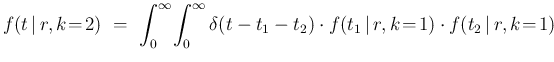
- It is interesting
to note that there is an alternative
way to get Eq. (),
starting from the joint distribution
 and then marginalizing it.
In fact, using the chain rule, we get
and then marginalizing it.
In fact, using the chain rule, we get
But, being
deterministically related
to and ,
 is nothing but
 (see also other examples in Ref. [1]).
Integrating then
over and we get Eq. ().
(see also other examples in Ref. [1]).
Integrating then
over and we get Eq. ().
.
.
.
.
.
.
.
.
.
.
.
.
.
.
.
.
.
.
.
.
.
.
.
.
.
.
.
.
.
.
- ... exponentially,28
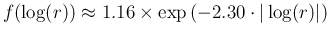
- Empirically,
we can evaluate, taking two points form the
histogram of Fig. ,
the following exponential:
 .
.
.
.
.
.
.
.
.
.
.
.
.
.
.
.
.
.
.
.
.
.
.
.
.
.
.
.
.
.
.
.
- ...
equations:29
- Perhaps it is worth noticing again
(see footnote ),
since this observation seems raised for the first time in this paper, that
Eq. () can be seen
not only as an extension to continuous variables of Eq. (),
but also as the joint pdf
 obtained by the
chain rule, that is
obtained by the
chain rule, that is
 ,
where
,
where
 ,
followed by marginalization.
,
followed by marginalization.
.
.
.
.
.
.
.
.
.
.
.
.
.
.
.
.
.
.
.
.
.
.
.
.
.
.
.
.
.
.
- ....30
- If
you like to reproduce the final result, given by Eq. ()
with Mathematica,
here are the commands to get it, although the output will appear a
bit cryptic (but you will recognize the resulting plot):
  rM = 10
  frho := Integrate[r2*DiracDelta[r1 - rho*r2]/rM^2, {r1, 0, rM}, {r2, 0, rM}]
  frho
  Plot[frho, {rho, 0, 5}]
.
.
.
.
.
.
.
.
.
.
.
.
.
.
.
.
.
.
.
.
.
.
.
.
.
.
.
.
.
.
- ... as31
- We can check
that
 , as previously guessed from symmetry arguments.
.
.
.
.
.
.
.
.
.
.
.
.
.
.
.
.
.
.
.
.
.
.
.
.
.
.
.
.
.
.
- ... simulations.32
- Curiously, this distribution
has the property that
 .
I wonder if there are others.
.
I wonder if there are others.
.
.
.
.
.
.
.
.
.
.
.
.
.
.
.
.
.
.
.
.
.
.
.
.
.
.
.
.
.
.
- ...
interest.33
- But when measuring rates, a flat prior
has more implications than one might think, as discussed in
chapter 13 of Ref. [13], and therefore
a full understanding of the physical case is desirable.
.
.
.
.
.
.
.
.
.
.
.
.
.
.
.
.
.
.
.
.
.
.
.
.
.
.
.
.
.
.
- ...,34
- Note that, since
priors are logically needed, programs of this kind require
them, even if they are flat. This can be seen as an annoyance,
but it is instead a power of these programs: first they can include
also non trivial priors; second, even if one wants to use flat
priors, the user is forced to think on the fact that priors are unavoidable,
instead of following the illusion
that she is using a prior-free method [42],
sometimes very dangerous, unless one does simple routine measurements
characterized by a very narrow likelihood [13].
.
.
.
.
.
.
.
.
.
.
.
.
.
.
.
.
.
.
.
.
.
.
.
.
.
.
.
.
.
.
- ... other.35
- At this point a clarification
is in order. When we make fits and say, again with reference to Fig. 1 of
Ref. [43], that the observations
 are independent from
each other we are referring to the fact that each depends
only on its
are independent from
each other we are referring to the fact that each depends
only on its  , e.g.
 ,
but not on the other
,
but not on the other
 . Instead,
the true values are
certainly correlated,
being
. Instead,
the true values are
certainly correlated,
being

 .
.
.
.
.
.
.
.
.
.
.
.
.
.
.
.
.
.
.
.
.
.
.
.
.
.
.
.
.
.
.
.
- ... which36
- Indeed, it can also be found
in the literature as the probability of the number of failures
before the first success occurs'
(for example, my preferred vademecum of Probability
Distributions, that is the
homonymous app [31],
reports both distributions).
.
.
.
.
.
.
.
.
.
.
.
.
.
.
.
.
.
.
.
.
.
.
.
.
.
.
.
.
.
.
- ... occurs.37
- Also of
this distribution there are
two flavors, the other one describing
the number of trials before the
 -th
success [31].
-th
success [31].
.
.
.
.
.
.
.
.
.
.
.
.
.
.
.
.
.
.
.
.
.
.
.
.
.
.
.
.
.
.
- ... instant38
- One could also think at `things'
occurring in `points' in some different space. All what we are going to
say in the domain of time can be translated in other domains.
.
.
.
.
.
.
.
.
.
.
.
.
.
.
.
.
.
.
.
.
.
.
.
.
.
.
.
.
.
.
- ... details,39
- It is indeed a useful exercise to
derive the Erlang distribution starting from
and going on until the general rule is obtained.
.
.
.
.
.
.
.
.
.
.
.
.
.
.
.
.
.
.
.
.
.
.
.
.
.
.
.
.
.
.
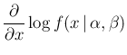
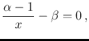
- ... maximum40
- Taking the log of
 , we get
the condition of maximum by
, we get
the condition of maximum by
resulting in
 .
.
.
.
.
.
.
.
.
.
.
.
.
.
.
.
.
.
.
.
.
.
.
.
.
.
.
.
.
.
.
.
 d
d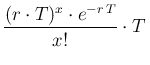 d
d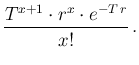
 d
d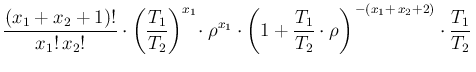 d
d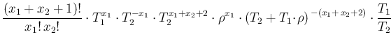 d
d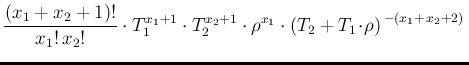 d
d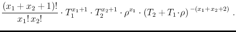
 d
d