Next: Conclusions Up: Use of MCMC methods Previous: Dependence of the rate
The first idea that might come to the mind is to apply the well known
weighted average of the individual values, using as weights the
inverses of the variances.
But, before doing it, it is important
to understand the assumptions behind it, that is something
that goes back to none other than Gauss, and for which
we refer to Refs. [29,44].
The basic idea of Gauss was to get two numbers (let us say
`central value' and standard deviation
- indeed Gauss used, instead of the standard deviation,
what he called `degree of precision' and
`degree of accuracy' [44], but
this is an irrelevant detail) such that
they contain the same information of the individual values.
In practice the rule of combination had to satisfy what
is currently known as statistical sufficiency.
Now it is not obvious at all that the weighted average
using
E![]() and
and
![]() satisfies sufficiency
(see e.g. the puzzle proposed in the Appendix of Ref. [44]).
satisfies sufficiency
(see e.g. the puzzle proposed in the Appendix of Ref. [44]).
Therefore, instead of trying to apply the weighted average
as a `prescription', let us see what comes out applying
consistently the rules of probability on a suitable model,
restarting from that of Fig. ![[*]](crossref.png) .
It is clear that if we consider meaningful a
combined value of
.
It is clear that if we consider meaningful a
combined value of ![]() for all
instances of
for all
instances of
![]() it means we assume
it means we assume
![]() not depending on a quantity
not depending on a quantity ![]() .
However,
.
However, ![]() could. This implies that the values of
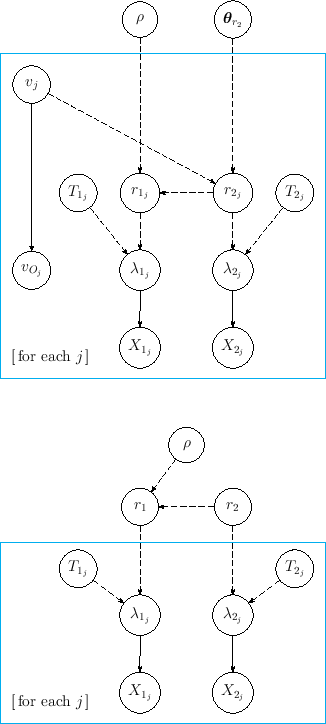
could. This implies that the values of ![]() are strongly correlated to each other.35Therefore the graphical model
of interest would be that at the top of Fig. .
are strongly correlated to each other.35Therefore the graphical model
of interest would be that at the top of Fig. .
A trivial case is when both rates, and therefore their ratio, are assumed
to be constant, although unknown, yielding then
the graphical model shown in the bottom diagram of
Fig. , whose related joint pdf, evaluated
by the best suited chain rule, is an extension of
Eqs. ()-()
![$\displaystyle \left[\,\prod_{j=1}^N f(x_{2_j}\,\vert\,r_2,T_{2_j})\right]\!\cdo...
...})\right]
\!\cdot\! f(r_1\,\vert\,r_2,\rho)\!\cdot\! f_0(\rho)\,,\ \ \ \ \ \ \ $](img584.png) |
(142) |
![$\displaystyle \left[\,\prod_{j=1}^N r_2^{x_{2_j}}\,
\cdot e^{-T_{2_j}\,r_2}\rig...
...}\,r_1}\right]\!\cdot
\delta(r_1-\rho\cdot r_2)\cdot f_0(\rho) \ \ \ \ \ \ \ \ $](img585.png) |
(143) | ||
| (144) |
),
with if we use the
total numbers of counts in the total times of measurements.
This is a simple and nice result, close to the intuition,
but we have to be aware of the model on which it is based.