Use of MCMC methods to cross-check the closed results and to analyze extended models

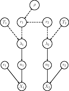
So far our models have been rather simple, missing however several real life complications. For example, assuming that we do observe the number of counts due to a Poisson distribution with a given $\lambda=r\cdot T$ clearly implies that we are neglecting efficiency issues. In order to include efficiencies we need to modify our graphical model of Fig.

(hereafter we stick to this last model), adding the relevant nodes.

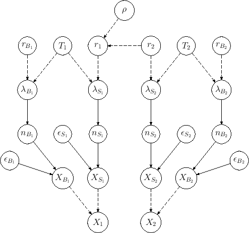
The extended model is shown in Fig. ,

**Figure:** *Extension of the model of Fig. in order to include efficiencies.*
$\begin{figure}\begin{center} \epsfig{file=inf_r2_rho_eff.eps,clip=,width=0.53\linewidth} \\ \mbox{} \vspace{-1.0cm} \mbox{} \end{center} \end{figure}$

in which we have redefined the symbols, keeping

and

associated to the observed counts and then calling

and

those `produced' by the Poissonians. Each

is then binomially distributed with parameters

and $\epsilon_i$ . In summary, listing the `causal relations' from bottom to top, we have

$\displaystyle X_i$	$\displaystyle \sim$	Binom $\displaystyle (n_i,\epsilon_i)$	(120)
$\displaystyle n_i$	$\displaystyle \sim$	Poisson $\displaystyle (\lambda_i)$	(121)
$\displaystyle \lambda_i$	$\displaystyle =$	$\displaystyle r_i\cdot T_i$	(122)
$\displaystyle r_1$	$\displaystyle =$	$\displaystyle \rho\cdot r_2$	(123)

At this point we can easily build up the joint distribution of all quantities in the network, as we have done in the previous section, and then evaluate the (possibly joint) distribution of the variables of interest, conditioned by those which are observed or somehow assumed. Moreover, also the efficiencies $\epsilon_1$ and $\epsilon_2$ are by themselves uncertain, and then we have to integrate also over them, taking into account their probability distributions $f(\epsilon_1)$ and $f(\epsilon_2)$ . In fact, their value come from test experiments or, more likely, from Monte Carlo simulations of the physics process and of the detector. So we need to enlarge the model adding four other nodes, taking into account the probabilistic links

$\displaystyle X_i^{(MC)}$

$\displaystyle \sim$

Binom $\displaystyle (n_i^{(MC)},\epsilon_i)\,.$

(124)

We refrain from adding the four nodes in the network of Fig.

, which will become more busy in a while. Anyway, we can just assign to $\epsilon_1$ and $\epsilon_2$ the parameter of the probability distribution resulting from the inferences based on Monte Carlo simulations (see Ref. [1] for details - remember that, having the nodes $\epsilon_1$ and $\epsilon_2$ no parents, they need priors).

What is still missing in the model of Fig. is background. In fact, we do not only lose events because of inefficiencies, but the `experimentally defined class' can get contributions from other `physical class(es)' (in general there are several physical classes contributing as background). Figure shows the extension

**Figure:** *Extended model of Fig. including also background.*
$\begin{figure}\begin{center} \epsfig{file=inf_r2_rho_eff_bkg.eps,clip=,width=0.89\linewidth} \\ \mbox{} \vspace{-1.2cm} \mbox{} \end{center} \end{figure}$

of the previous model, in which each Poisson process which describes the signal has just one background Poisson process. All variables have subscripts

, depending if their are associated to signal or background (with exception of

and

, which are obviously the two signal rates). As before, the nodes needed to infer the efficiencies are not shown in the diagram, which is therefore missing eight `bubbles'.

At this point it is clear that trying to achieve closed formulae is out of hope, and we need to use other methods to perform the integrals of interest, namely those based on Markov Chain Monte Carlo. We show here how to use a powerful package that does the work for us. But we do it only for the two cases of which we already have closed solutions in hand, that is the models of Figs. and starting from uniform priors for the `top nodes'. The program we are going to use is JAGS [36] interfaced to R via the package jrags [37].

Introducing MCMC and related algorithms goes well beyond the purpose of this paper and we recommend Ref. [38] (some examples of application, including R scripts, are also provided in Ref. [1]). Moreover, mentioning the Gibbs Sampler algorithm applied to probabilistic inference (and forecasting) it is impossible not to refer to the BUGS project [39], whose acronym stands for Bayesian inference using Gibbs Sampler, that has been a kind of revolution in Bayesian analysis, decades ago limited to simple cases because of computational problems (see also Sec. 1 of Ref.[36]). In the BUGS project web site [40] it is possible to find packages with excellent Graphical User Interface, tutorials and many examples [41].

Subsections