Model B (Fig. ), with flat priors on and

Model B (Fig. ), with flat priors on $\rho$ and

Let us move to the model of Fig.

, whose implementation in the JAGS language is the following:

model {
  x1 ~ dpois(lambda1)
  x2 ~ dpois(lambda2)
  lambda1 <- r1 * T1
  lambda2 <- r2 * T2
  r1 <- rho * r2
  r2  ~ dgamma(1, 1e-6)
  rho ~ dgamma(1, 1e-6)
}

The complete R script, which uses the same data ( $x_1\!=\!3,\,T_1\!=\!3\,$ s; $x_2\!=\!6,\,T_2\!=\!6\,$ s) is provided in Appendix B.6. The result is shown in Fig.

and the details are given in the following printouts

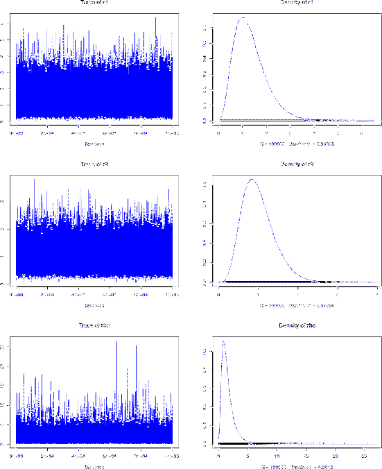**Figure:** *Graphical summary of the chain produced by the script of Appendix B.6 implementing the graphical model of Fig. .*
$\begin{figure}\begin{center} \epsfig{file=jags_model_2.eps,clip=,width=\linewidth} \\ \mbox{} \vspace{-1.2cm} \mbox{} \end{center} \end{figure}$

1. Empirical mean and standard deviation for each variable,
   plus standard error of the mean:

     Mean     SD Naive SE Time-series SE
r1  1.334 0.6694 0.002117       0.002117
r2  1.002 0.4068 0.001286       0.001925
rho 1.595 1.1918 0.003769       0.006058

2. Quantiles for each variable:

      2.5%    25%    50%   75% 97.5%
r1  0.3616 0.8438 1.2234 1.704 2.941
r2  0.3671 0.7061 0.9477 1.238 1.940
rho 0.3167 0.8199 1.2923 2.012 4.638

Exact:
   r1 =  1.333 +- 0.667
   r2 =  1.000 +- 0.408
  rho =  1.600 +- 1.200

Again, the agreement between the MCMC and the exact results is excellent.