Direct inference of the rate ratio $\rho$ (and of $r_2$)

We have remarked several times that $r_1$ and $r_2$ are inferred from the observed numbers of events $X_1$ and $X_2$ (we assume $T_1$ and $T_2$ can be exactly known), and that the possible values of their ratio $\rho$ are successively evaluated (`deduced') from each possible pair of values of the rates. This logical scheme is represented by the graphical model of Fig. . But this is not the only way to approach the problem. 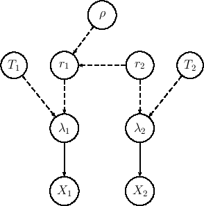An alternative model is shown in Fig. ,

Figure: Alternative graphical model to that of Fig. .

in which the node $\rho$ appears `at the top' of the network and it is then really inferred <sup>26</sup>(indeed also $r_2$ is `at the top', having above it no parents nodes from which to depend).

Writing one diagram or another one is not just a question of drawing art. Indeed, the network reflects the supposed causal model (`what depends from what') and therefore the choice of the model can have an effect on the results. It is therefore important to understand in what they differ. In the model of Fig.  the rates $r_1$ and $r_2$ assume a primary role. We infer their values and, as a byproduct, we get $\rho$. In this new model, instead, it is $\rho$ to have a primary role, together with one of the two rates (they cannot be both at the same level because there is a constraint between the three quantities). Our choice to make $r_1$ depend on $r_2$ is due to the fact that $r_2$, appearing at the denominator, can be seen as a `baseline' to which the other rate is referred (obviously, here $r_1$ and $r_2$ are just names, and therefore the choice of their role depend on their meaning).

The strategy to get $f(\rho\,\vert\,\ldots)$ is then different, being this time $\rho$ directly inferred using the Bayes theorem applied to the entire network. A strong advantage of this second model is that, as we shall see, its prior can be factorized (see also Ref. [1], especially Appendix A there, in which there is a summary of the formulae we are going to use).

In analogy to what has been done in detail in Ref. [1], the pdf of $\rho$ is obtained in two steps: first infer $f(\rho,r_1,r_2\,\vert\,x_1,x_2,T_1,T_2)$; then get the pdf of $\rho$ by marginalization. For the first step we need to write down the joint distribution of all variables in the network (apart from $T_1$ and $T_2$ which we consider just as fixed parameters, having usually negligible uncertainty) using the most convenient chain rule, obtained navigating bottom up the graphical model. Indicating, as in Ref. [1], with $f(\ldots)$ the joint pdf of all relevant variables, we obtain from the chain rule

$$f(\ldots) = f(x_2\,\vert\,r_2,T_2)\cdot f_0(r_2)\cdot f(x_1\,\vert\,r_1,T_1) \cdot f(r_1\,\vert\,r_2,\rho)\cdot f_0(\rho)\,\,$$ (78)

from which we can get, besides a normalization constant, the pdf's of interest as

$$f(\rho\,\vert\,x_1,T_1,x_2,T_2) \propto \int_0^\infty\!\!\!\int_0^\infty\! f(\ldots) \, r_1\, r_2$$ (79)

$$f(r_2\,\vert\,x_1,T_1,x_2,T_2) \propto \int_0^\infty\!\!\!\int_0^\infty\! f(\ldots) \, \rho\, r_1\,,$$ (80)

or the joint pdf $f(r_2,\rho\,\vert\,x_1,T_1,x_2,T_2)$, integrating only over $r_1$. Using explicit expressions of the pdf's, of which $f(r_1\,\vert\,r_2,\rho)$ is just the Dirac delta $\delta(r_1\!-\!\rho\cdot r_2)$,²⁷and ignoring multiplicative factors, we can then only focus on

$$\tilde f(\ldots) \!\! \propto r_2^{x_2} \cdot e^{-T_2\,r_2}\cdot f_0(r_2) \cdot r_1^{x_1} \cdot e^{-T_1\,r_1}\cdot \delta(r_1-\rho\cdot r_2)\cdot f_0(\rho)\,,$$ (81)

having indicated by $\tilde f()$ the unnormalized pdf.