For completeness, let us also try to get the closed expressions
of
 and
and
 , although only under the assumption
of a flat prior of
, although only under the assumption
of a flat prior of  . In this case this choice is forced
from the fact that
. In this case this choice is forced
from the fact that
 cannot be expressed in term of a conjugate prior
which would then simplify the calculations. For the general case, in fact,
we have to change methods, moving to Markov Chain
Monte Carlo (MCMC), as done e.g.
in Ref. [1] and as it will be sketched in the next section.
cannot be expressed in term of a conjugate prior
which would then simplify the calculations. For the general case, in fact,
we have to change methods, moving to Markov Chain
Monte Carlo (MCMC), as done e.g.
in Ref. [1] and as it will be sketched in the next section.
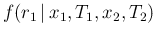
In order to get the pdf of  , we need to restart from
the unnormalized joint distribution (
, we need to restart from
the unnormalized joint distribution (![[*]](crossref.png) ),
proceeding then like in Eq. (),
but this time integrating over
),
proceeding then like in Eq. (),
but this time integrating over  and
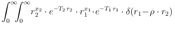
and absorbing the constant priors in the proportionality factor:
and
and absorbing the constant priors in the proportionality factor:
 |
 |
 d d d d |
(108) |
| |
|
 d d d d |
(109) |
| |
|
 d d d d |
(110) |
| |
|
 d d |
(111) |
| |
|
 |
(112) |
thus reobtaining, besides normalization,
Eq. ().
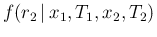
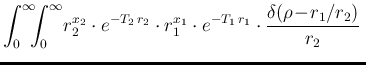
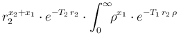
Similarly, we have
 |
|
d d |
(113) |
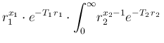
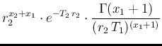
| |
|
d d |
(114) |
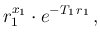
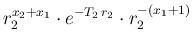
| |
|
 d d |
(115) |
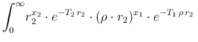
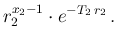
| |
|
 d d |
(116) |
| |
|
 |
(117) |
| |
|
 |
(118) |
| |
|
 |
(119) |
We see that, differently from
,
the power of is, instead of  ,
,  ,
that is we get an effect similar to that found for the
distribution of . As a consequence, expected values
and standard deviation of are
,
that is we get an effect similar to that found for the
distribution of . As a consequence, expected values
and standard deviation of are  and
and
 , respectively.