The very essence of the so called probabilistic
inference (`Bayesian inference')
is given by Eq. (![[*]](crossref.png) ).
The rest is just a question of normalization and of
extending it to the continuum, that in our case of interest is
).
The rest is just a question of normalization and of
extending it to the continuum, that in our case of interest is
It is evident the symmetric role of
 and
and
 , if the former is seen
as a mathematical function of
, if the former is seen
as a mathematical function of  for a given (`observed')
 , that is playing the role of a parameter.
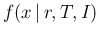
This function is known as likelihood and commonly indicated by
, that is playing the role of a parameter.
This function is known as likelihood and commonly indicated by
 .19Indicating the second factor of
Eq. (), that is the `infamous' prior
that causes so much anxiety in practitioners [8],
by
.19Indicating the second factor of
Eq. (), that is the `infamous' prior
that causes so much anxiety in practitioners [8],
by  , we get (assuming
  implicit, as it is
usually the case)
implicit, as it is
usually the case)
which makes it clear that we have two mathematical functions of
playing symmetric and
peer roles. Stated in different words,
each of the two has the role of `reshaping'
the other [1].
In usual `routine' measurements
(as watching your weight on a balance) the information provided
by
 is so much narrower, with
respect to
is so much narrower, with
respect to
 ,20that we can neglect the latter and absorb it
in the proportionality factor, as we have done above
in Sec. . Employing a uniform
`prior' is then usually a good idea to start with,
unless
arises from previous measurements
or from strong theoretical prejudice on the quantity
of interest. It is also very important to understand that
`the reshaping' due to the priors can be done
in a second step, as it has been pointed out, with
practical examples, in Ref. [1].
,20that we can neglect the latter and absorb it
in the proportionality factor, as we have done above
in Sec. . Employing a uniform
`prior' is then usually a good idea to start with,
unless
arises from previous measurements
or from strong theoretical prejudice on the quantity
of interest. It is also very important to understand that
`the reshaping' due to the priors can be done
in a second step, as it has been pointed out, with
practical examples, in Ref. [1].
Let us now see what happens when, in our case, the
Bayes rule is applied in sequence in order to account for
several results on the same
rate , that is assumed to be stable.
Imagine we start from rather vague ideas about the value of ,
such that  is, in practice, the best
practical choice we can do. After
the observation of
is, in practice, the best
practical choice we can do. After
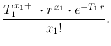
the observation of  counts during
  we get,
as we have learned above,
we get,
as we have learned above,
Then we perform a new campaign of observations
and record  counts in
  . It is clear now that in the second
inference we have to use as `prior'
the piece of knowledge derived from the first inference.
So, we have, all together, besides irrelevant factors,
. It is clear now that in the second
inference we have to use as `prior'
the piece of knowledge derived from the first inference.
So, we have, all together, besides irrelevant factors,
that is exactly as we had done a single experiment,
observing
 counts in
 .
The only real physical strong assumption is that the intensity
of Poisson process was the same during the two measurements,
i.e. we have being measuring the same thing.
.
The only real physical strong assumption is that the intensity
of Poisson process was the same during the two measurements,
i.e. we have being measuring the same thing.
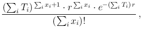
This teaches us immediately how to `combine the results',
an often debated subject
within experimental teams, if we have sets of counts  during times
  (indicated all together by '
 ' and `
 '):
'):
without imaginative averages or fits. But this does not mean
that we can blindly sum up counts and measuring times.
Needless to say, it is important, whenever it is possible,
to make a detailed study of the
behavior of
 in order to
be sure that the intensity is compatible with being constant
during the measurements. But, once we are confident about its constancy
(or that there is no strong evidence against that hypothesis),
the result is provided by Eq. (),
from which all summaries of interest can be derived.21
in order to
be sure that the intensity is compatible with being constant
during the measurements. But, once we are confident about its constancy
(or that there is no strong evidence against that hypothesis),
the result is provided by Eq. (),
from which all summaries of interest can be derived.21