Next: Conjugate priors Up: Inferring and ( possibly Previous: Role of the priors
![[*]](crossref.png) )
and focus on the role of the likelihood to reshape
)
and focus on the role of the likelihood to reshape
To be clear, let us make the example of
having observed zero counts, that is
the experiment was indeed performed, but no event of interest
was found during the measurement time ![]() .
If we use a flat prior and
only stick to the summaries, we have that the most probable
value is zero, with
E
.
If we use a flat prior and
only stick to the summaries, we have that the most probable
value is zero, with
E![]() :
the larger is the measuring time, the more the distribution
of
:
the larger is the measuring time, the more the distribution
of ![]() is squeezed towards zero.
But this does not give a complete picture of what is going on.
Since
is squeezed towards zero.
But this does not give a complete picture of what is going on.
Since
![]() goes to 1 for
goes to 1 for
![]() ,
the likelihood is opened in the left side.
Figure shows
,
the likelihood is opened in the left side.
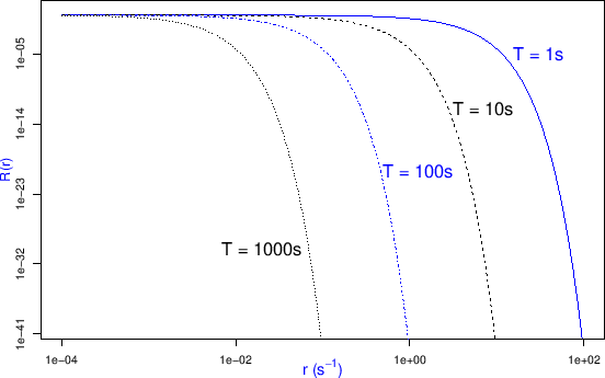
Figure shows ![]()
If we run the experiment longer and longer,
keeping observing zero events, the possible values of ![]() gets smaller and smaller. What is mostly interesting,
in this plot, is the region in which
gets smaller and smaller. What is mostly interesting,
in this plot, is the region in which ![]() is flat: it means
that if our beliefs are concentrate there, then
the experiment does not teach us more than what we already believed:
the experiment looses sensitivity in that region
and then reporting `probabilistic' upper limits makes no sense
and it can be highly misleading (even more reporting `C.L.
upper limits`) [13,27].
is flat: it means
that if our beliefs are concentrate there, then
the experiment does not teach us more than what we already believed:
the experiment looses sensitivity in that region
and then reporting `probabilistic' upper limits makes no sense
and it can be highly misleading (even more reporting `C.L.
upper limits`) [13,27].