At this point a technical remark is in order. The reason
why the Gamma appears so often is that the expression of
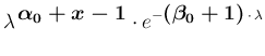
the Poisson probability function, seen as a function of  and neglecting multiplicative factors,
that is
and neglecting multiplicative factors,
that is
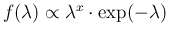 ,
has the same structure of a Gamma pdf.
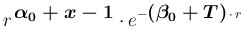
The same is true if the variable
,
has the same structure of a Gamma pdf.
The same is true if the variable  is considered,
that is
is considered,
that is
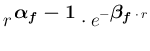
 . If
then we have a Gamma distribution as prior, with parameters
. If
then we have a Gamma distribution as prior, with parameters
 and
and  , the `final' distributions is still a
Gamma:
, the `final' distributions is still a
Gamma:
This kind of distributions, such that the `posterior' belongs to
the same family of the `prior', with updated parameters,
are called conjugate priors for obvious reasons,
as it is rather obvious how convenient they are
in applications,
provided they are flexible enough to describe `somehow'
the prior belief.24 This was particularly important at the times
when the monstrous computational power nowadays available
was not even imaginable
(also the development of logical and mathematical
tools has a strong relevance).
Therefore a quite rich
collection of conjugate priors
is available in the literature (see e.g. Ref. [30]).
In sum, these are the updating rules of the Gamma parameters
for our cases of interest (the subscript ' ' is to remind
that is the parameter of the `final' distribution):
' is to remind
that is the parameter of the `final' distribution):
(Note that in the case of the parameter  has the dimension
of a time, being a rate, that is counts per unit of time.)
A flat prior distribution is recovered for
has the dimension
of a time, being a rate, that is counts per unit of time.)
A flat prior distribution is recovered for
 and
and
 .
Technically,
for
.
Technically,
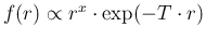
for  a Gamma distribution turns into a negative exponential:
if then the `rate parameter' is chosen to be
very small, the exponential
becomes `essentially flat' in the region of interest.
a Gamma distribution turns into a negative exponential:
if then the `rate parameter' is chosen to be
very small, the exponential
becomes `essentially flat' in the region of interest.
Once we have learned the updating rules
(![[*]](crossref.png) )-()
and ()-(),
it might be convenient to turn a prior expressed in terms
of mean
)-()
and ()-(),
it might be convenient to turn a prior expressed in terms
of mean  and standard deviation
  into
and , inverting the expressions of
expected value and standard deviation of a Gamma distributed
variable (see Appendix A), thus getting
into
and , inverting the expressions of
expected value and standard deviation of a Gamma distributed
variable (see Appendix A), thus getting
For example, if we have good reason to think that
should be
 s
s , the parameters
of our initial Gamma distribution are
, the parameters
of our initial Gamma distribution are
 and
and
 s. This is equivalent to having
started from a flat prior and having observed (rounding the numbers)
5 counts in about 1.2 seconds. This gives a clear idea of the
`strength' of the prior - not much in this case, but it certainly
excludes the possibility of
s. This is equivalent to having
started from a flat prior and having observed (rounding the numbers)
5 counts in about 1.2 seconds. This gives a clear idea of the
`strength' of the prior - not much in this case, but it certainly
excludes the possibility of  . This happens in fact
as soon as is larger then 1, implying
. This happens in fact
as soon as is larger then 1, implying
 vanishing at .
This observation can be a used as a trick to forbid a vanishing value
of or of , if we have good physical reason
to believe that they cannot be zero, although we are
highly uncertain about even their order of magnitude:
just choose a prior slightly larger than one.
vanishing at .
This observation can be a used as a trick to forbid a vanishing value
of or of , if we have good physical reason
to believe that they cannot be zero, although we are
highly uncertain about even their order of magnitude:
just choose a prior slightly larger than one.