Inference of  given
given  , assuming

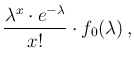
The probability density function of is evaluated
from the so called Bayes' rule:
where
 is the so called
`prior'.9 Assuming for the moment
a `flat' prior, that is
is the so called
`prior'.9 Assuming for the moment
a `flat' prior, that is
 ,
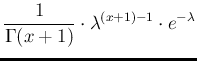
and neglecting
all factors non depending on , we get
,
and neglecting
all factors non depending on , we get
in which we recognize a Gamma pdf with
 and
and  (see Appendix A - for a detailed derivation
see e.g. Ref. [13]), and therefore
(see Appendix A - for a detailed derivation
see e.g. Ref. [13]), and therefore
Expected value, standard deviation and mode are
 ,
,
 and , respectively.
The advantage of having expressed the distribution of
in terms of a Gamma is that we can use the
probability distributions made available from programming languages, e.g.
in R, which usually include also useful random generators
(e.g. rgamma() in R). For example,
making use of the R function dgamma()
we can draw
Fig.
and , respectively.
The advantage of having expressed the distribution of
in terms of a Gamma is that we can use the
probability distributions made available from programming languages, e.g.
in R, which usually include also useful random generators
(e.g. rgamma() in R). For example,
making use of the R function dgamma()
we can draw
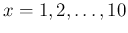
Fig. ![[*]](crossref.png) ,
,
Figure:
Inferred
 , using a flat prior,
for
, using a flat prior,
for
 .
.
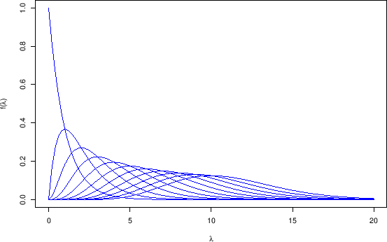 |
which shows
, for
 , with the following
few lines of code:
, with the following
few lines of code:
for (x.o in 0:10) {
  curve(dgamma(x,x.o+1,1),xlim=c(0,20),ylim=c(0,1),col='blue',add=x.o>0,
        xlab=expression(lambda),ylab=expression(paste('f(',lambda,')')))
}