Next: Distribution of the ratio Up: Inferring Poisson 's and Previous: Inference of given ,
x1 = 1
x2 = 1
lambda1 = rgamma(n, x1+1, 1)
lambda2 = rgamma(n, x2+1, 1)
rho = lambda1/lambda2
Then, varying x1 and x2 we can get the plots of Figs.
![[*]](crossref.png) and .10
and .10
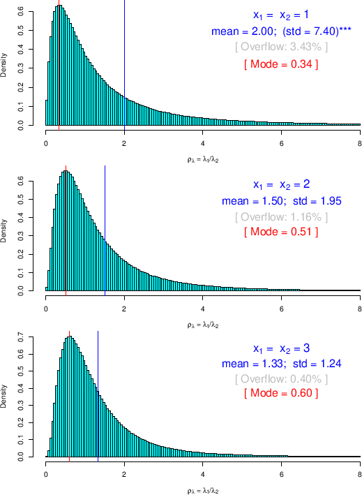 |
The effect of the long tails is that there is quite a big difference
between mean value and the most probable one, located around the
highest bar of the histogram. This
is not a surprise (the famous exponential distribution
has modal value equal to zero independently of its parameter!),
but it should sound as a warning for those who use analysis methods
which provide, as `estimator',
“the most probable value”11 [13].
Moreover,
for very small ![]() the tails do not seem to
go very fast to zero (in comparison e.g. to the exponential),
leading to not-defined moments of the distribution
(of the theoretical one, obviously,
since in most cases mean and standard deviation
of the Monte Carlo distribution have finite values).
This question will be investigated
in the next subsection, after the derivation
of closed expressions.
the tails do not seem to
go very fast to zero (in comparison e.g. to the exponential),
leading to not-defined moments of the distribution
(of the theoretical one, obviously,
since in most cases mean and standard deviation
of the Monte Carlo distribution have finite values).
This question will be investigated
in the next subsection, after the derivation
of closed expressions.
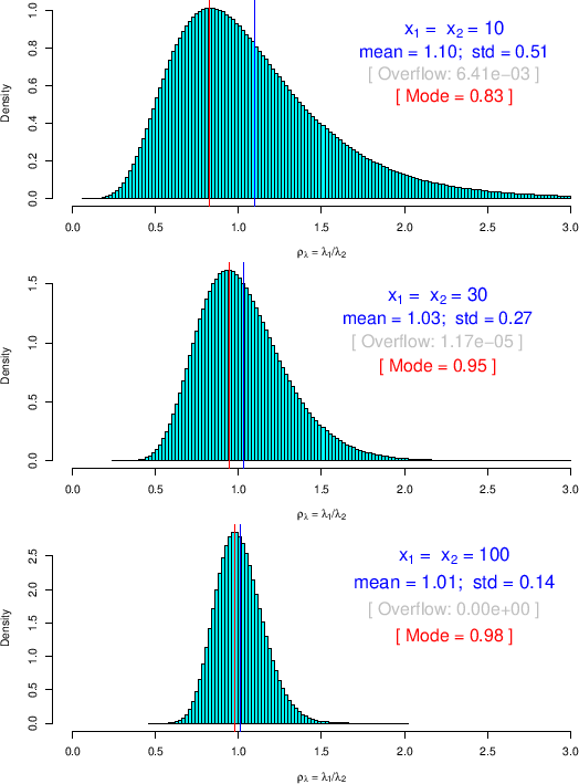
When ![]() and
and ![]() become `quite large' the Gamma distribution
tends (slowly - think to the
become `quite large' the Gamma distribution
tends (slowly - think to the ![]() , that is
indeed a particular Gamma, as
reminded in Appendix A) to a Gaussian, and likewise does
(a bit slower) the ratio of two Gamma variables
(as
, that is
indeed a particular Gamma, as
reminded in Appendix A) to a Gaussian, and likewise does
(a bit slower) the ratio of two Gamma variables
(as ![]() and
and ![]() are), as we can see for the case
are), as we can see for the case
![]() of
Fig. ,12in which some skewness is still visible and the mode is
about
of
Fig. ,12in which some skewness is still visible and the mode is
about ![]() smaller than the mean value.
smaller than the mean value.