Distribution of the ratio of Poisson  's in closed form
Being the evaluation of ratio of rates (to which the ratio of
's is related)
an important issue in Physics, it is worth trying to get
an analytic expression for its pdf.
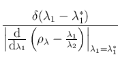
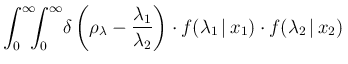
This can be done extending to the continuum
Eq. (![[*]](crossref.png) ),13that is replacing the sums
by integrals, and applying the constraint between the
two variables by a Dirac delta [13]:
),13that is replacing the sums
by integrals, and applying the constraint between the
two variables by a Dirac delta [13]:
Making use of the properties of the  , we can rewrite it as
with
 root of the equation
 ,
and therefore equal to
,
and therefore equal to
 . Equation
() becomes then
. Equation
() becomes then
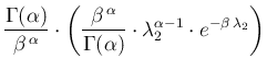
Once more we recognize in the integrand something related
to the Gamma distribution. In fact, identifying the power of  with `
 ' of a Gamma pdf, and `
 ' at the exponent
with the `rate parameter'
' at the exponent
with the `rate parameter'  , that is
the integrand in Eq. () can be rewritten as
in order to recognize within parentheses a Gamma pdf
in the variable , whose integral over
is then equal to one because of normalization. We get then
The mode of the distribution can be easily obtained
finding the maximum (of the log) of the pdf, thus getting
in agreement with what we have got in Figs.
and by Monte Carlo
(indeed, done there in a fast and rather rough way - see Appendix B.2).
In order to get expected value and standard deviation, we need
to evaluate the relevant integrals14
- First we check that
 is properly
normalized. Indeed the integral
is properly
normalized. Indeed the integral
 d
d is equal to unity
for `all possible'
is equal to unity
for `all possible'  and
and  .15
.15
- The expected value is equal to
in perfect agreement with what we can read
from the Monte Carlo results of Figs.
and .
- The expected value of
 is given by
from which we evaluate
(subtracting to it the square of the expected value)
from which the standard deviation follows,
that we rewrite in a more compact form
as
having indicated by
 the expected value
of
.
For the values and used in Figs.
and , we get, starting from
the expected value
of
.
For the values and used in Figs.
and , we get, starting from
 in increasing order, the following
standard deviations: 1.936, 1.247, 0.507, 0.269 and 0.143,
in agreement with the Monte Carlo results (or the other way around).
in increasing order, the following
standard deviations: 1.936, 1.247, 0.507, 0.269 and 0.143,
in agreement with the Monte Carlo results (or the other way around).
The detailed comparison between closed expression of the pdf
and the Monte Carlo outcome is shown in
Fig. for the toughest case
we have met, that is  .
.
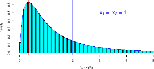
Figure:
Comparison of the distribution of
 obtained by the closed expression
() with that
estimated by Monte Carlo (same as top plot of
Fig. ). The vertical
lines indicate mode and expected value, evaluated
using Eqs. () and
(), equal to 1/3 and 2, respectively.
(Note that none of these values is close to 1, that is what
one would naively expect for the ratio of the rates - indeed, only for
and above
obtained by the closed expression
() with that
estimated by Monte Carlo (same as top plot of
Fig. ). The vertical
lines indicate mode and expected value, evaluated
using Eqs. () and
(), equal to 1/3 and 2, respectively.
(Note that none of these values is close to 1, that is what
one would naively expect for the ratio of the rates - indeed, only for
and above
 mode, expected value
and ratio of the observed counts become approximately equal).
mode, expected value
and ratio of the observed counts become approximately equal).
 |
 d
d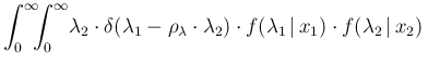 d
d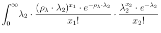 d
d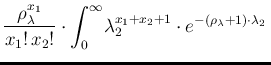 d
d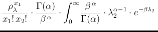 d
d