Next: Final distributions of and Up: Direct inference of the Previous: Inferred distribution of
![[*]](crossref.png) , yielding
Eq. () starting from
, yielding
Eq. () starting from
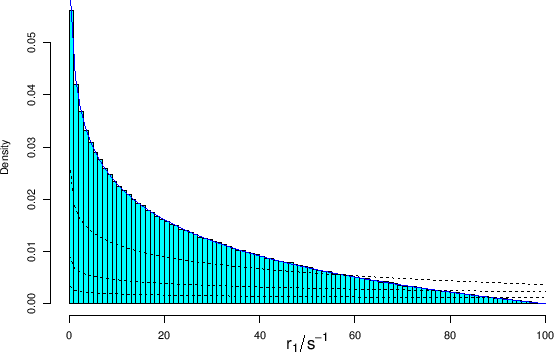
n = 10^7
rM = 100
r1 = runif(n, 0, rM)
r2 = runif(n, 0, rM)
rho = r1/r2
rho.h <- rho[rho<5]
hist(rho.h, nc=200, col='blue', freq=FALSE)
abline(v=1, col='red')
where the selection of the values below
(a more complete script, which also
performs the correct normalization of the histogram,
is shown in Appendix B.4).
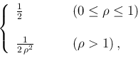
The histogram is characterized by
a plateau till 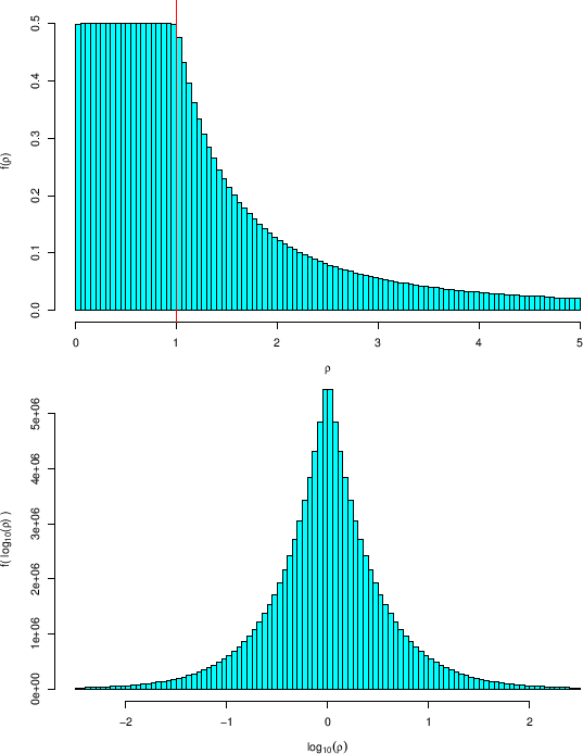 |
Although it might be bizarre, this histogram shows in essence
the prior on ![]() we have been tacitly assumed,
when flat priors on
we have been tacitly assumed,
when flat priors on ![]() and
and ![]() were chosen (as a cross check,
the commented instructions of the script of Appendix B.4, executed one by
one, plot the distribution of
were chosen (as a cross check,
the commented instructions of the script of Appendix B.4, executed one by
one, plot the distribution of ![]() assuming
a flat prior for
assuming
a flat prior for ![]() and the curious distribution of
the top plot of
Fig. for
and the curious distribution of
the top plot of
Fig. for ![]() ).
).
In order to have a better insight of what is going on,
the bottom plot of the same figure shows the histogram
of
![]() . The maximum is at
. The maximum is at
![]() and it decreases symmetrically, exponentially,28as
and it decreases symmetrically, exponentially,28as
![]() increases.
This symmetry indicates that the probabilities
to get a value of
increases.
This symmetry indicates that the probabilities
to get a value of ![]() below or above 1 are the same.
The same conclusion, within the uncertainties
due to sampling, can be drawn from the histogram in linear scale,
since
below or above 1 are the same.
The same conclusion, within the uncertainties
due to sampling, can be drawn from the histogram in linear scale,
since ![]() is `about
is `about ![]() ' for
' for
![]() . Similarly,
from the comparison of the two histograms we can
evaluate, by symmetry arguments, that the probability that
. Similarly,
from the comparison of the two histograms we can
evaluate, by symmetry arguments, that the probability that
![]() is between 0.1 and 10 is equal to 90% (exact value, indeed
as we shall see in a while).
is between 0.1 and 10 is equal to 90% (exact value, indeed
as we shall see in a while).
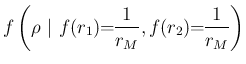
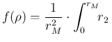
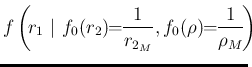
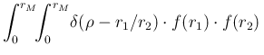
It is interesting to get the distribution shown
in the top plot of
Fig. making a transformation
of variables, as we have done in Eq. () and following
equations:29
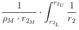
At this point, some care is needed with the limits of the integral
over ![]() , due to its `natural' upper limit at
, due to its `natural' upper limit at ![]() and to that
given by the constraint
and to that
given by the constraint
![]() , i.e.
, i.e.
![]() .
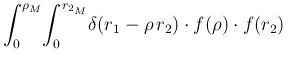
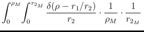
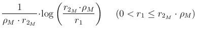
Therefore, after the trivial integration over
.
Therefore, after the trivial integration over ![]() , we are left with
, we are left with
 d d |
(102) |
 d d |
|||
 d d |
For completeness, let also make the game of seeing how
flat priors on ![]() and
and ![]() (up to
(up to ![]() and
and ![]() , respectively)
are reflected into
, respectively)
are reflected into ![]() in the model of Fig.:
in the model of Fig.:
 d d |
(104) | ||
 d d |
(105) | ||
 d d |
(106) |
 |
 |
||
| |
(107) |
 |
,
in which the exact pdf (blue solid line)
is compared with the Monte Carlo result.
The plot also shows the pdf's of ,
the model of Fig. can accommodate
in practice flat prior distributions for the three quantities of
interest.33
 d
d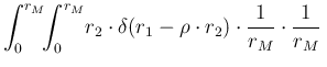 d
d