Next: More on the ratio Up: Ratio of Gamma distributed Previous: Ratio of Gamma distributed
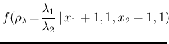
![[*]](crossref.png) , we get,
applying Eq. () and
writing the conditions in terms of the Gamma parameters,
).
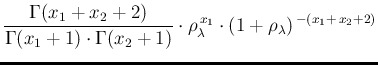
, we get,
applying Eq. () and
writing the conditions in terms of the Gamma parameters,
).
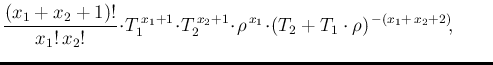
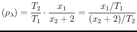
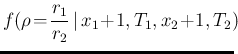
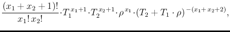
As far as the ratio of rates, starting again from a uniform prior,
implying then
![]() and
and
![]() ,
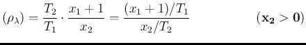
we get,
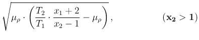
writing, as in Eq. (),
the conditions in terms of the Gamma parameters,
,
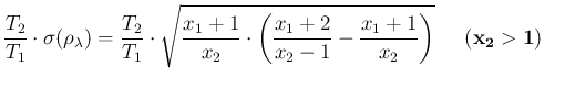
we get,
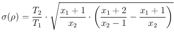
writing, as in Eq. (),
the conditions in terms of the Gamma parameters,
 |
 |
) and
()
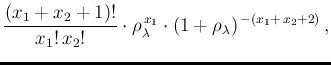
in the special case )-(),
just noting that
 |
 |
 |
(66) |
and
,
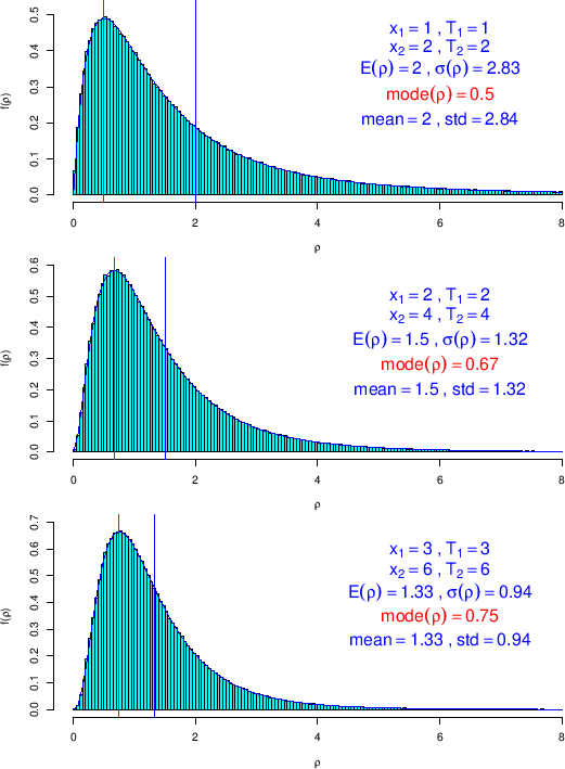
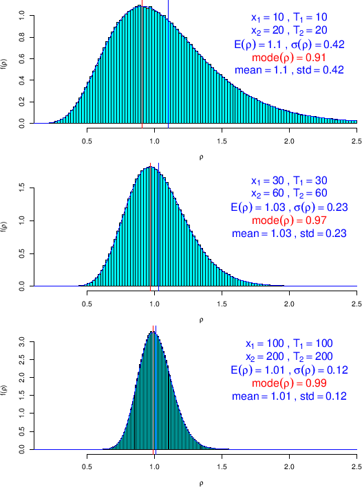
for low and relatively high
numbers of counts, respectively.
Each plot shows
both the curve of the pdf, calculated with the closed formulae
just derived,
and the histogram of Monte Carlo simulation
(the script to reproduce these plots is given in Appendix B.3).
The value of mode, expected value and standard
deviation calculated from exact formulae are reported too,
together with `mean' and `std' (`empirical standard deviation')
evaluated from the sampling. The excellent agreement can be
considered a cross check of the exact formulae, derived above for
the purpose.
The counts and the measuring times have been chosen such that
![]() are equal to one in all cases.
Therefore the plots are comparable to those of
Figs.
and reporting
are equal to one in all cases.
Therefore the plots are comparable to those of
Figs.
and reporting
![]() for several values of
for several values of
![]() (but in that case all summaries were evaluated from sampling,
having, at that stage of the work, not yet derived
the closed formulae of interest). As we can again see,
for small numbers of counts the distribution of the ratio of rates
is strongly asymmetric, with mode and expected value
systematically below and above, respectively,
the ratio calculated naively as
(but in that case all summaries were evaluated from sampling,
having, at that stage of the work, not yet derived
the closed formulae of interest). As we can again see,
for small numbers of counts the distribution of the ratio of rates
is strongly asymmetric, with mode and expected value
systematically below and above, respectively,
the ratio calculated naively as
![]() .
This value is reached asymptotically, as we see in
Fig. , and as expected by the fact
that for high numbers of counts we get
.
This value is reached asymptotically, as we see in
Fig. , and as expected by the fact
that for high numbers of counts we get
mode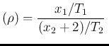 |
 |
(67) | |
E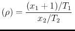 |
|
(68) | |
 |
(69) |