Keeping the notation  for the ratio of the generic
Gamma distributed variables
for the ratio of the generic
Gamma distributed variables  and
and  , the pdf
of Eq. (
, the pdf
of Eq. (![[*]](crossref.png) ) can be further
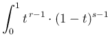
simplified reminding that the beta
special function (or Euler integral of the
first kind [33]), defined as
) can be further
simplified reminding that the beta
special function (or Euler integral of the
first kind [33]), defined as
can be written as
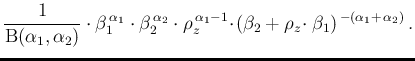
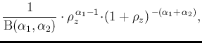
We can then rewrite the combination of three gamma
functions appearing in Eq. ()
as
 B
B ,
thus getting
,
thus getting
As far as mode, expected value and variance are concerned,
they can be obtained, without direct calculations,
just transforming those of
 , seen above,
remembering that, starting from a flat prior,
, seen above,
remembering that, starting from a flat prior,
 Gamma
Gamma .
We get then
.
We get then
mode |
 |
 |
(73) |
| |
|
|
|
| E |
|
 |
(74) |
| |
|
|
|
| Var |
|
![$\displaystyle \frac{\beta_2^2}{\beta_1^2}\cdot
\left[ \frac{\alpha_1}{\alpha_2-...
...\frac{\alpha_1}{\alpha_2-1}\right)\right]
\hspace{0.85cm}(\mathbf{\alpha_2>2}).$](img351.png) |
(75) |
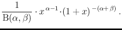
Moreover, just for completeness, let us mention
the special case
 , that
written for the generic variable
, that
written for the generic variable  , becomes
`known' (certainly not to me before I was
attempting to write these subsection)
as Beta prime distribution [34],
with parameters  and
and  :
:
The name of the distribution is clearly due to the special function
resulting from normalization. It is `prime'
in order to distinguish it
from the more famous (and more important as far as
practical applications are concerned)
Beta distribution which arises quite `naturally' when inferring
the parameter  of the Bernoulli trials, in the light of
 successes in
  trials (essentially the original problem
tackled by Bayes [19] and Laplace [20]),
and then used as conjugate
prior of the binomial distribution
(see e.g. Ref. [30] as well as
Ref. [1] for practical applications).
The Beta prime distribution
is actually what has been independently derived in
Sec. to describe
trials (essentially the original problem
tackled by Bayes [19] and Laplace [20]),
and then used as conjugate
prior of the binomial distribution
(see e.g. Ref. [30] as well as
Ref. [1] for practical applications).
The Beta prime distribution
is actually what has been independently derived in
Sec. to describe
 , although
the beta special function was not used there,
nor in Sec. .
, although
the beta special function was not used there,
nor in Sec. .
 d
d