Model A (Fig. ), with flat priors on and

We start from the model of Fig.

. The code that instructs JAGS about the model is practically a transcription of the expressions to state that a variable follows a given distribution. Therefore, since we have

$\displaystyle X_1$	$\displaystyle \sim$	Poisson $\displaystyle (\lambda_1)$	(125)
$\displaystyle X_2$	$\displaystyle \sim$	Poisson $\displaystyle (\lambda_2)$	(126)
$\displaystyle \lambda_1$	$\displaystyle =$	$\displaystyle r_1\cdot T_1$	(127)
$\displaystyle \lambda_2$	$\displaystyle =$	$\displaystyle r_2\cdot T_2$	(128)
$\displaystyle \rho$	$\displaystyle =$	$\displaystyle r_1/r_2\,,$	(129)

we get

model {
  x1 ~ dpois(lambda1)
  x2 ~ dpois(lambda2)
  lambda1 <- r1 * T1
  lambda2 <- r2 * T2
  r1 ~ dgamma(1, 1e-6) 
  r2 ~ dgamma(1, 1e-6)
  rho <- r1/r2
}

in which are also included the flat priors of

and

,³⁴implemented by Gamma distributions with $\alpha=1$ and $\beta\lll 1$ :

$\displaystyle r_1$	$\displaystyle \sim$	Gamma $\displaystyle (1, 10^{-6})$	(130)
$\displaystyle r_2$	$\displaystyle \sim$	Gamma $\displaystyle (1, 10^{-6})$	(131)

The complete R script which calls rjags and shows the results is provided in Appendix B.5 (see Ref. [1] for clarifications about the structure of the R code).

**Figure:** *Graphical summary of the chain produced by the script of Appendix B.5 implementing the graphical model of Fig. .*
$\begin{figure}\begin{center} \epsfig{file=jags_model_1.eps,clip=,width=\linewidth} \\ \mbox{} \vspace{-1.2cm} \mbox{} \end{center} \end{figure}$

The values of ( $x_1\!=\!3,\,T_1\!=\!3\,$ s) and ( $x_2\!=\!6,\,T_2\!=\!6\,$ s) have been chosen in order to have small numbers, but with finite expected values and standard deviation, in order to make a comparison with the results of the closed formulae. The parameter determining the `length' of the Markov chain has been set at

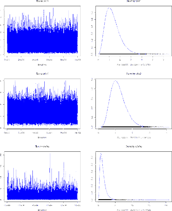The summary figure , drawn automatically by R when the command plot() is called with first argument an MCMC chain object, shows, for each of the three variables that we have chosen to monitor, the `trace' and the 'density'. The latter is a smoothed representation of the histogram of the possible occurrences of a variable in the chain. The former shows the `history' of a variable during the sampling, and it is important to understand the quality of the sampling. If the traces appear quite randomic, as they are in this figure, there is nothing to worry. Otherwise we have to increase the length of the chain so that it can visit each `point' (in fact a little volume) of the space of possibilities with relative frequencies `approximately equal' to their probabilities (just Bernoulli theorem, nothing to do with the `frequentist definition of probability').

Here is the relevant output of the script:

1. Empirical mean and standard deviation for each variable,
   plus standard error of the mean:

     Mean     SD Naive SE Time-series SE
r1  1.334 0.6671 0.002110       0.002110
r2  1.167 0.4418 0.001397       0.001397
rho 1.333 0.9444 0.002986       0.002986

2. Quantiles for each variable:

      2.5%    25%   50%   75% 97.5%
r1  0.3637 0.8457 1.223 1.700 2.927
r2  0.4701 0.8481 1.111 1.424 2.179
rho 0.2772 0.7048 1.102 1.684 3.770

Exact:
   r1 =  1.333 +- 0.667
   r2 =  1.167 +- 0.441
  rho =  1.333 +- 0.943

As we can see, the agreement between the MCMC and the exact results, evaluated from Eqs. (

) and (

), is excellent (remember that `r1 = 1.333 +- 0.667' stands for E $(r_1)=1.333\,$ s $^{-1}$ and $\sigma(r_1)=0.667\,$ s $^{-1}$ ).