Comparison of the results from the two models

An overall comparison of the two models, again based on the observations of 3 counts in 3 s from process 1 and 6 counts in 6 s from process 2, is shown in Fig. ,

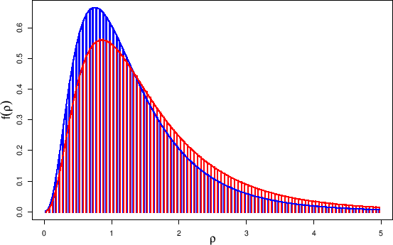
Figure: Comparison of the distribution of $\rho=r_1/r_2$ obtained by the models of Fig.  (blue, slightly narrower) and Fig.  (red, slightly wider) in the case of ( $x_1=3,T_1=3\,$s) and ( $x_1=6,T_1=6\,$s) using flat priors for the top nodes. The histograms are the JAGS results and the lines come from the pdf's in closed form (see text).

while expected values and standard deviations (separated by `$\pm$') calculated from the closed formulae are summarized in the following table.

	Model A (Fig. )	Model B (Fig. )
	$[\,f_0(r_1)\!=\!k\ \& \ f_0(r_2)\!=\!k\,]$	$[\,f_0(\rho)\!=\!k\ \&\ f_0(r_2)\!=\!k\,]$
$r_1\,($s$^{-1})$	$1.33\pm 0.67$	$1.33\pm 0.67$
$r_2\,($s$^{-1})$	$1.17\pm 0.44$	$1.00\pm 0.41$
$\rho$	$1.33\pm 0.94$	$1.60\pm 1.20$

As we have seen in Fig. , the second model produces a distribution of $\rho$ with higher expected value and higher standard deviation.