Next: Combining ratios of rates Up: Use of MCMC methods Previous: Comparison of the results
| (132) |
| (133) |
![[*]](crossref.png) to that of Fig.
to that of Fig.
 |
| Poisson |
(134) | ||
| Poisson |
(135) | ||
| (136) | |||
| (137) | |||
| (138) | |||
| (139) | |||
| (140) |
The priors which are easier to choose
are those of ![]() , if their values are `well measured',
that is if
, if their values are `well measured',
that is if
![]() are small enough.
We can then confidently use flat priors, as done e.g.
for the `unobserved'
are small enough.
We can then confidently use flat priors, as done e.g.
for the `unobserved' ![]() of Fig. 1 in Ref. [43].
of Fig. 1 in Ref. [43].
Also the priors about
![]()
![]() can be
chosen quite vague, paying however some care
in order to forbid negative values of
can be
chosen quite vague, paying however some care
in order to forbid negative values of ![]() .
Incidentally, having mentioned the simple case of linear
dependence, an important sub-case is when
.
Incidentally, having mentioned the simple case of linear
dependence, an important sub-case is when ![]() is assumed to be null: the remaining
prior on
is assumed to be null: the remaining
prior on ![]() becomes indeed the prior on
becomes indeed the prior on ![]() ,
and the inference of
,
and the inference of ![]() corresponds to the
inferred value of
corresponds to the
inferred value of ![]() having taken into account
several instances of
having taken into account
several instances of ![]() and
and ![]() - this is indeed the question
of the `combination of values of
- this is indeed the question
of the `combination of values of ![]() ' on which we
shall comment a bit more in detail in the sequel.
' on which we
shall comment a bit more in detail in the sequel.
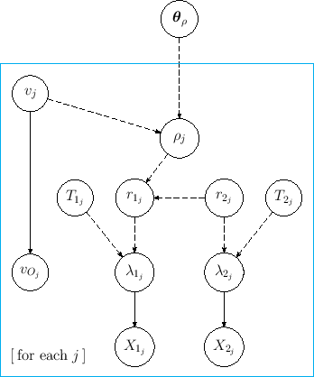
As far as the priors of the rates are concerned,
one could think, a bit naively, that the choice of independent
flat priors for ![]() could be a reasonable choice.
But we need to understand the physical model underlying this choice.
In fact, most likely, as the ratio
could be a reasonable choice.
But we need to understand the physical model underlying this choice.
In fact, most likely, as the ratio ![]() might depends on
might depends on ![]() , the same
could be true for
, the same
could be true for ![]() , but perhaps with a completely
different functional dependence.
For example
, but perhaps with a completely
different functional dependence.
For example ![]() and
and ![]() could have a strong
dependence on
could have a strong
dependence on ![]() , e.g. they could decrease exponentially,
but, nevertheless, their ratio could be independent of
, e.g. they could decrease exponentially,
but, nevertheless, their ratio could be independent of ![]() ,
or, at most, could just exhibit a small linear dependence.
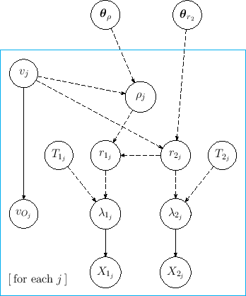
Therefore we have to add this possibility into the model,
which then becomes as in Fig. ,
,
or, at most, could just exhibit a small linear dependence.
Therefore we have to add this possibility into the model,
which then becomes as in Fig. ,
 |
| (141) |
At this point, any further consideration goes beyond the rather general purpose of this paper, because we should enter into details that strongly depend on the physical case. We hope that the reader could at least appreciate the level of awareness that these graphical models provide. The existence of computing tools in which the models can be implemented makes then nowadays possible what decades ago was not even imaginable.